%%{init: {"theme": "base", "themeVariables": {"primaryColor": "#E8ECFF", "primaryBorderColor": "#4054B2", "primaryTextColor": "#16171B", "lineColor": "#3B4351", "edgeLabelBackground": "#FAF7F0", "clusterBkg": "#EFE9DC", "clusterBorder": "#766F65"}, "flowchart": {"rankSpacing": 26, "nodeSpacing": 32}}}%%
flowchart TB
  subgraph TRAIN["Training --- centralised"]
    direction LR
    G["Global state +<br/>joint actions"] --> K["Central critic"]
    K -->|"credit signal"| P1["π₁"]
    K --> P2["π₂"]
    K --> P3["π₃"]
  end
  subgraph EXEC["Execution --- decentralised"]
    direction TB
    O1["local obs o₁"] --> Q1["π₁"] --> A1["action a₁"]
    O2["o₂"] --> Q2["π₂"] --> A2["a₂"]
    O3["o₃"] --> Q3["π₃"] --> A3["a₃"]
    KX["✗ critic absent<br/>at execution"]
  end
  TRAIN ==>|"only the policies ship"| EXEC
  classDef world fill:#EFE9DC,stroke:#766F65,color:#16171B
  class KX world
17 Learning in Multi-Agent Systems
Part IV closed with its own confession: every institution it built was designed for players who stay put. This chapter withdraws the assumption, and the withdrawal is not a small perturbation — it changes the character of everything. A single agent learning alone faces a stationary problem: the world has fixed habits, the agent improves against them, and a well-stocked theory guarantees that patience will be rewarded. Add one more learner and the guarantee quietly dies. Each agent’s training signal is now generated partly by the other’s behaviour, so each agent’s improvement is the other’s distribution shift: the coder learns to write code the reviewer approves, while the reviewer is learning new grounds for disapproval, and both are aiming at targets that move because they are being aimed at. The ground learns back. Everything distinctive about multi-agent learning — its instabilities, its strange dynamics, its occasional spectacular triumphs — follows from that one sentence.
A word on what “learning” means here, because for this book’s agents it happens at three timescales at once. Slowest, the weights: training and fine-tuning, where the classical theory lives. Faster, the context: a language model adapts within a single conversation by conditioning on what has happened (Chapter 3), no gradient required. And in between, the memory: an agent that accumulates notes, retrieves precedents, and revises its own playbook (Chapter 7) is learning in every sense an engineer should care about, one deployment at a time. (A statistician may prefer adaptation for the umbrella, reserving learning for changed parameters; nothing below depends on the label, because what carries across the timescales is structure, not theorems.) The results in this chapter were mostly discovered in the gradient world, but the structure — moving targets, credit that must be assigned, curricula that generate themselves, rules that get gamed — recurs at all three timescales, which is why a book about foundation-model agents needs this chapter even though none of its readers is likely to train a Go engine.
The subject’s pedigree is distinguished and, at its origin, familiar: the founding formalism of multi-agent learning, the stochastic game, was published by Shapley in 1953 — the same year as his value, which was evidently a good year at Princeton. The field built outward from there: reinforcement learning generalised to Markov games; decentralised cooperation was formalised and promptly shown to be computationally savage; and self-play — the trick of letting an agent be its own opponent — carried machine play from backgammon to Go to the great e-sports demonstrations, some of the most famous results in the history of artificial intelligence, every one of them a multi-agent learning story. The present twist is that the largest single-agent models are themselves products of multi-agent training: a policy and a reward model locked in their instructive little dance, self-generated data curricula, models grading models. Multi-agent learning is no longer a corner of the field. It is the water.
One stipulation, inherited from the preface and honoured throughout: this is a conceptual chapter. Teaching multi-agent reinforcement learning properly requires building value functions, policy gradients, and a good deal of deep learning first, and the book that does so already exists, is excellent, and is free — we shall point to it repeatedly and without resentment. What this chapter keeps is the map and the connections: the four ideas that recur through the rest of the book — non-stationarity, multi-agent credit assignment, self-play, and emergent communication, the learned twin of Chapter 8’s designed protocols — and the genuinely contemporary question that Part VI will inherit: whether coordination among capable agents should be learned or composed. We proceed from the moving-target problem itself (Section 17.1); to the formal ground — Markov games, and the Dec-POMDP that completes Chapter 11’s partial-observability story at a bracing complexity class (Section 17.2); to credit assignment and the compromise that made cooperative learning practical (Section 17.3); to the two things learning invents when left to its own devices — opponents and languages (Section 17.4); and finally to the learned-or-composed question, posed where Part IV’s institutions meet players that adapt to them (Section 17.5).
17.1 Moving Targets: Learning Among Learners
Everything that makes learning alone tractable can be put in one sentence: the world does not care that you are learning. A lone agent improving by trial and error is running statistics on a process with fixed habits — act, observe the consequence, update the estimate — and because the consequences are drawn from distributions that hold still, patience pays: estimates sharpen, behaviour improves, and under conditions the classical theory makes precise, the improvement provably converges on the best available. That theory — built on Bellman’s Markov Decision Process, which the reader met briefly in Section 6.3 and which this book deliberately declines to construct — is one of the quiet triumphs of the field, and its every guarantee rests on the same load-bearing clause. The world may be stochastic, hostile, even mostly unobservable; what it may not do is rearrange itself in response to being learned about.
That is, of course, exactly what another learner does. Put a second adapting agent in the system and, from each agent’s chair, the other is simply part of “the environment” — but an environment that is now running the same manoeuvre in reverse: studying you, updating on you, redistributing its behaviour because of what you have lately been doing. The stationarity clause is not bent but broken, and broken by construction rather than by accident, because the violation is the setting: a multi-agent system whose members adapt is, definitionally, a system in which everyone’s training data is generated by everyone else’s ongoing revision. This is non-stationarity, the first of the chapter’s recurring ideas, and its structure deserves a careful sentence: each agent is doing statistics on a data-generating process that its own statistics are changing, through the medium of the other agents’ learning. The loop has no privileged fixed point supplied for free. Whatever stability the system finds, it must find on its own.
The canonical demonstration costs one afternoon and repays it. Take a repeated two-player game — a small coordination game will do — and let each player run standard single-agent learning while treating the other as scenery: what Tan, in the paper that named the arrangement, called independent learners (1993). Sometimes this simply works, which is the maddening part, because it works often enough to lull. And often it produces the signature pathology: pursuit. Agent A adapts to B’s current habit; the adaptation changes A’s behaviour; B, learning from a world that contains A, revises; A’s hard-won estimates now describe an opponent that no longer exists, and the pair orbit the solution without settling on it — each learning, neither converging, both perpetually well-adapted to the other’s recent past. The subtle version of the same disease afflicts any agent that learns from stored experience: a memory buffer of episodes against last week’s counterpart is archaeology — lovingly curated data about a vanished civilisation — and the more efficiently the agent mines it, the more precisely it fits what is gone. The chapter’s lab makes the orbit visible; a page of prose cannot compete with watching it.
What exactly breaks divides into three losses and, importantly, one gain. The guarantees go first: convergence theorems condition on stationarity, so among learners they simply do not apply — not “apply more weakly”, do not apply. Evaluation goes next, and more quietly: “better” becomes opponent-indexed, since a policy is only better or worse against someone, so yesterday’s improvement can be today’s regression with no one having blundered — a relativity that Chapter 24 will meet as a measurement problem and Section 17.4 as a strategic one. Third, legibility becomes a liability: an agent that adapts in a predictable way can be farmed by a faster or subtler learner, which turns the innocent business of improvement into the strategic business of Chapter 12 — learning about learners is itself a game. The gain is the flip side of the same coin, and the chapter’s later optimism depends on it: a target that moves just ahead of the learner is not a pathology but a teacher, and arranging for the moving target to move helpfully — curriculum by opponent — is the trick behind the field’s greatest successes, of which more in Section 17.4. The surveys that organised the field are organised around this ledger of losses and gains (Buşoniu et al., 2008), and the reader who wants the full taxonomy of remedies, with the mathematics this chapter forgoes, should go where the preface pointed: the field’s dedicated textbook covers it from foundations (Albrecht et al., 2024), the first of several such referrals, made without resentment.
One family of guarantees, and essentially only one, survives the wreckage, and its shape is instructive. An agent can bound its regret — the gap between the reward its choices earned and what the best fixed alternative would have earned in hindsight — against any sequence of opponent behaviour whatsoever, because the guarantee never assumed a stationary world in the first place; and when every player learns under that discipline, something collective emerges from the purely individual promise: the time-averaged record of joint play converges — not to a Nash equilibrium, but to the correlated equilibria or their coarser cousins, depending on the strength of regret being driven down (Foster & Vohra, 1997; Hart & Mas-Colell, 2000). That is the honest trade written as a theorem: convergence among learners can be had, but the solution concept weakens under you — the destination is a broader, laxer set than the one single-agent optimisation was promised. The pattern deserves memorising, because it is this book’s thesis in miniature: what survives the passage from one agent to many is real, and it is always less than what was packed.
None of this is quarantined in the gradient world, and here the chapter earns its place in a book about foundation-model agents. Learning happens to our agents at three timescales. At the slowest, weights change: training and fine-tuning, where the classical results live. At the fastest, context changes: two language-model agents in one conversation adapt to each other turn by turn — each message conditions the other’s next — which is non-stationarity operating inside a single context window, with no gradient anywhere in sight. And between them sits memory (Chapter 7): an agent that accumulates a playbook, retrieves precedents, and revises its own notes is learning at deployment speed, one episode at a time. A team of frozen-weight models with persistent memories is therefore a multi-agent learning system in every sense that matters: the coder’s accumulated style guide shifts what the reviewer sees, the reviewer’s remembered objections shift what the coder writes, and the pair chase each other’s revisions just as the Q-learners chase each other’s habits — with the sobering difference that for memory-timescale learning there is, as yet, no convergence theory at all. Engineers run these systems anyway, which is not a criticism; it is the reason the structural lessons of the gradient era are worth carrying over. They are the only map of this territory anyone has.
| Timescale | Cadence | Mechanism | Gradient? | Convergence theory |
|---|---|---|---|---|
| Weights | Slowest | Training and fine-tuning | Yes | Classical single-agent theory; among learners, only the no-regret family (Section 17.1) |
| Context | Fastest — turn by turn, within one window | Condition on the conversation so far (Chapter 3) | No | None |
| Memory | In between — one deployment at a time | Accumulate a playbook, retrieve precedents, revise one’s own notes (Chapter 7) | No | None, as yet |
The rest of the chapter is the field’s set of answers, and they slot into a sentence apiece. If other learners break your world model, adopt a world model in which other learners are first-class citizens — the formal ground of Markov games and the Dec-POMDP (Section 17.2). If the team learns as one but is scored as one too, fix the signal, so that credit lands on the member who earned it (Section 17.3). If the moving target is the problem, choose the target — make the opponent yourself, and turn drift into curriculum (Section 17.4). And if none of the guarantees on offer covers the coordination you need, decline to learn it: compose it from Part III and Part IV’s machinery instead, a choice that deserves an explicit rubric rather than a default (Section 17.5). First, the formal ground — where the moving target gets a mathematics.
17.2 The Formal Ground: Markov Games and the Dec-POMDP
The first remedy for a broken world model is a better world model: if other learners violate your assumptions, adopt a formalism in which other learners are not interference but inhabitants. That formalism has existed since before reinforcement learning did. A Markov game — Shapley called it a stochastic game, and defined it in the same 1953 the chapter’s opening admired (1953) — can be read in two directions, both illuminating. Read from Chapter 12, it is a matrix game given scenery: the players’ joint action determines not only their payoffs but the next state, so the game they play next depends on how they played this one. Read from the reinforcement-learning side, it is an MDP given company: the transitions and rewards respond to a joint action, so “the environment” now contains other strategists by construction rather than by embarrassment. Shapley defined the model to prove that zero-sum stochastic games have well-defined values — decades before there was anything resembling machine learning to run on it, in what the reader will recognise as this book’s oldest running joke played absolutely straight.
The frame’s first dividend is a taxonomy, because reward structure decides what “solving” even means. Fully cooperative Markov games — every agent paid identically — pose a pure team problem: find the best joint policy, hard for reasons about to become vivid but at least well-posed. Fully competitive (two-player zero-sum) games are Shapley’s original case, and the cleanest: a value exists, worst-case play is well-defined, and the single-agent learning machinery generalises with its dignity largely intact — Littman’s minimax-Q, the paper that installed Markov games as the field’s standard frame, did that generalisation (1994). Everything else — general-sum games, which is to say almost everything real — imports Chapter 12’s troubles wholesale: equilibria multiply, selection among them is unresolved, and “solving the game” quietly becomes “choosing which equilibrium to hope for”. The taxonomy is worth internalising because it prices ambition: the same algorithm that provably converges in a zero-sum game merely runs in a general-sum one.
One more honest admission completes the frame. The Markov game still assumes that every player observes the state — the whole board, everyone’s position, all of it. Chapter 11 spent its entire length on why teams do not enjoy this luxury: views are local, state is partial, and nobody sees the whole. The model that takes both facts seriously at once — shared goal, joint dynamics, private views — is the Dec-POMDP: a decentralised, partially observable Markov decision process, in which a team earns a common reward while each member receives only its own observations and must act on nothing more than its own history of them (Oliehoek & Amato, 2016). A policy here is not a plan over states — no agent has the state — but a mapping from each agent’s private history to its next action, and communication, where it exists at all, is an action: something with a cost and a timing, not a free window onto teammates’ minds. This is the formal completion of Chapter 11’s theme, and the starred treatment this book defers to its apparatus lives here: the Dec-POMDP is the canonical mathematics of what an orchestrated team of partially informed agents actually is.
Then comes the theorem that calibrates the whole enterprise. Bernstein and colleagues proved that solving a finite-horizon Dec-POMDP optimally is NEXP-complete (2002) — and the reader who does not keep complexity classes on the mantelpiece should hear the scale in plain words. NP-hard problems, this book’s usual villains, can at least have their candidate solutions checked cheaply. Single-agent partial observability is harder still — PSPACE-complete — which the planning community had learnt to live with. NEXP sits above both: under standard assumptions the brute-force cost is doubly exponential, and the result holds for two agents, tiny horizons, everything finite and known. The jump from one decision-maker to two, under partial observability, is not a doubling of difficulty. It is a change of complexity class — the price of decentralisation written as a theorem, and a fact worth quoting whenever a whiteboard diagram makes distributed autonomy look like a deployment detail.
Why should two be so much worse than one? Because the agents have lost the one thing that makes partial observability tractable alone: a shared summary of what is known. A single POMDP agent can maintain a belief state — a running distribution over where things stand — and act on it. A Dec-POMDP team has no common belief to maintain: each member’s belief is conditioned on its own private history, so acting well requires reasoning about what teammates have seen, which requires reasoning about what they believe, which requires reasoning about what they believe you have seen — Chapter 9’s nested beliefs, no longer a philosophical curiosity but the load-bearing structure of the planning problem. The exponential stack of histories-about-histories is precisely where the second exponential comes from. The Russian dolls, it turns out, were the complexity class.
17.2.1 The Markov Game and the Dec-POMDP, Formally*
The two frames deserve their tuples. A Markov game among n agents N = \{1, \dots, n\} is
\langle N, \mathcal{S}, \{A_i\}_{i \in N}, T, \{r_i\}_{i \in N}, \gamma \rangle,
where \mathcal{S} is the set of states; A_i is agent i’s action set, with joint actions A = A_1 \times \cdots \times A_n; T : \mathcal{S} \times A \to \Delta(\mathcal{S}) gives a probability distribution over next states, \Delta(X) denoting the set of probability distributions over X; r_i : \mathcal{S} \times A \to \mathbb{R} is agent i’s reward; and \gamma \in [0, 1) is the discount (reinforcement learning’s \gamma is the economics chapters’ \delta — both conventions are standard). The joint action is where the strategy lives: transitions and rewards answer to what everyone did. Set n = 1 and the tuple is Bellman’s MDP; shrink \mathcal{S} to a single state and it is one of Chapter 12’s repeated games — the section’s two readings of the model, recovered as special cases.
The Dec-POMDP amends this in three places, one informational, one motivational, and one clerical: each agent acquires a private observation set \Omega_i, with an observation function O : \mathcal{S} \times A \to \Delta(\Omega_1 \times \cdots \times \Omega_n) dealing every member its own partial glimpse of each state; the several rewards r_i merge into one shared r : \mathcal{S} \times A \to \mathbb{R}; and the discount \gamma goes, because the model will be run to a finite horizon rather than for ever — so that the whole reads
\langle N, \mathcal{S}, \{A_i\}_{i \in N}, T, r, \{\Omega_i\}_{i \in N}, O \rangle,
a team with common pay and private eyes. Since no agent sees the state, no agent can hold a policy over states: agent i’s policy is a map \pi_i : \Omega_i^{*} \to A_i from its private observation history — the sequence of everything it has personally seen — to its next action, and a joint policy is one such map per member. Bernstein’s theorem, with its hypotheses in full: given a Dec-POMDP over finite sets, with n \ge 2 agents, a finite horizon shorter than the number of states, and a threshold K, deciding whether any joint policy achieves expected total reward at least K is NEXP-complete (2002). Every hypothesis earns its keep — at n = 1 the same decision problem is PSPACE-complete; drop the short-horizon assumption and only the hardness half of the result survives; and note that this is only the decision version: certifying that a good enough joint policy exists already costs the class, and finding one is no cheaper.
17.2.2 Escape Routes
Hardness results are signposts, not stop signs, and this one points somewhere specific: since exact decentralised optimality is unattainable, everything practical must buy the problem down, and the purchasable currencies are the themes of this book. Communication is the first: let the agents talk freely and cheaply, and the team collapses toward a single centralised problem — merely PSPACE-hard, which in this neighbourhood counts as a bargain. Every message, in this light, is a purchase of tractability, and Chapter 8 and Chapter 11’s machinery is what the purchasing looks like. Offline centralisation is the second: even if execution must be decentralised, preparation need not be — plan or train with the global view, then distribute policies that run on local views alone, which is the CTDE compromise the next section examines. And pre-computed coordination is the third: Chapter 11’s conventions and Chapter 16’s roles are, in this frame, amortised planning — coordination decided once, offline, so that it need not be re-derived inside anyone’s exponential. The reader may also notice what the theorem says about the modern orchestrator: centralising the coordination in one context window is not a failure of architectural nerve. It is a rational escape from a complexity class.
The frames have now done what frames can do. The Markov game names the strategic difficulty and prices it by reward structure; the Dec-POMDP names the informational difficulty and prices it in complexity; between them they say why learning among learners is hard and where the escape routes run. What neither supplies is the thing a learning team needs next: a signal. A cooperative team is scored as a team — one reward, jointly earned — and gradient or no gradient, the lesson has to reach the member whose behaviour earned it. That is credit assignment, the chapter’s second recurring idea, and Chapter 16 has already supplied the instrument.
17.3 Whose Doing Was It? Credit and the CTDE Compromise
A cooperative team has one scoreboard, and that is the problem. The sprint ships, the suite scores 84 per cent, the whole team is paid the same number — and somewhere inside that number, the coder’s elegant refactor and the reviewer’s afternoon of rubber-stamping are indistinguishable. Hand every member the global reward as its learning signal and each agent’s actual contribution is drowned in the noise of everyone else’s: the idle agent is reinforced whenever its colleagues succeed — free-riding by gradient, no cynicism required — while the excellent agent is punished for blunders it never made. The statistics are as bad as they look: as the team grows, the correlation between any one member’s behaviour and the shared outcome shrinks, so learning from a team signal gets slower exactly as the team gets larger. This is multi-agent credit assignment, the chapter’s second recurring idea, and it is Chapter 16’s fair-division question with the sentiment stripped out: not who deserves the reward, but where the gradient should land.
The principled answer is the one the reader already owns. Chapter 16 established that “who contributed what” has a canonical solution — the Shapley value, marginal contribution averaged over arrival orders — and for an offline audit of four agents it costs sixteen benchmark runs, an afternoon. A learner cannot afford an afternoon per update; it needs the same quantity, or a serviceable shadow of it, at every step. The field’s workhorses are exactly such shadows. Difference rewards ask the one-agent counterfactual: what would the team have scored had this agent stayed home, or done something default and dull? — and reward each member on the difference, so that free-riding earns precisely nothing. COMA’s counterfactual baseline does the same surgery on actions rather than membership: marginalise out one agent’s action while holding everyone else’s fixed, and credit the agent with how much better its actual choice was than its average one (J. Foerster et al., 2018). The family resemblance is worth seeing plainly: each of these is a single slice of the Shapley computation — one term of the audit, evaluated cheaply where the full average cannot be — and the practical art of cooperative learning is largely the art of estimating Chapter 16’s quantity at training-loop prices.
| Method | The counterfactual it asks | Cost | Slice of the Shapley audit |
|---|---|---|---|
| Shapley value (Chapter 16) | Marginal contribution, averaged over arrival orders | Exact — 16 runs for four agents, an afternoon; unaffordable per update | The full average |
| Difference rewards | What the team would have scored had this agent stayed home, or done something default | Cheap — affordable at every update | One slice, by membership |
| Counterfactual baseline (COMA) (J. Foerster et al., 2018) | How much better this agent’s action was than its average, others held fixed | Cheap — affordable at every update | One slice, by action |
Computing such counterfactuals requires seeing the whole board, and thereby hangs the field’s standard architecture. Centralised training with decentralised execution (CTDE) splits the agent’s life into two regimes: during training, a centralised critic observes the global state and every agent’s action — which is what makes counterfactual credit computable at all — while the policies being trained consume only their own local observations; at deployment, the critic is dismantled like site scaffolding, and what ships is a set of policies that run on local views alone (J. Foerster et al., 2018; Lowe et al., 2017). The reader should hear Section 17.2 cashing its cheque — carefully, because the cheque is smaller than it looks. Exact decentralised optimisation is NEXP-hard, and centralising the training does not repeal that: the policies being sought still act on local views, so the search is the same search, attacked by gradient rather than solved. What the global view buys is the estimation inside the search — the counterfactuals of the previous paragraph become computable, because someone at last sees the whole board. The same privileged seat also softens Section 17.1’s non-stationarity during training: a critic that conditions on every agent’s action no longer watches its regression target drift as the others learn — though each policy still trains against teammates in motion, so the moving target is steadied for the valuer, not stopped for the learners. A related family factorises the team’s value into per-agent pieces so that each member can act greedily on its own share — the same instinct, applied to the value function itself. CTDE is not a theorem; it is a compromise. But it is the compromise on which most of modern cooperative multi-agent learning stands.
What the compromise can deliver, at its best, is coordination that was never written down anywhere. The line of work from Prorok’s laboratory at Cambridge is this book’s standing exhibit. Teams of robots learn decentralised control policies structured as graph neural networks: each robot’s policy computes over its local neighbourhood in the communication graph, so the network architecture is the communication topology, and the messages agents exchange are the network’s own learned representations — trained centrally, in simulation, with the global view; executed on physical robots over ad-hoc radio, each acting on what it and its neighbours can see (2022; 2020). The problems solved are Chapter 11’s own — multi-robot path planning, the corridor and the crossing, coverage and passage — but where Chapter 11 composed its solutions from locks, protocols, and conflict-based search, here the coordination is learned: no engineer specified who yields, and the deference emerges in the weights. When it works, it is quietly spectacular — coordination with no protocol document, running on hardware.
Heterogeneity sharpens the exhibit into a thesis. Real teams are not interchangeable — different sensors, different bodies, different jobs — and forcing every agent through one shared policy squanders exactly the differences that make a team worth having. Training genuinely heterogeneous policies that still coordinate — distinct behaviours, coupled through learned, differentiable communication — is the harder problem the HetGPPO line addresses (Bettini et al., 2023), and what is being learned is recognisable at sight: a division of labour, roles discovered by training rather than assigned by charter. The honest ledger from the same line of work, though, belongs in the same paragraph: learned coordination is data-hungry, simulation-bound until proven otherwise, and opaque in precisely the way composed coordination is not — there is no protocol document because there is no protocol, only weights, and Chapter 8’s auditability arguments do not evaporate merely because the results impress. That ledger is the seed of Section 17.5’s rubric.
None of this is robotics parochialism, because the credit problem does not care what the agents are made of. Fine-tune a multi-agent pipeline on team outcomes and the question is immediate: whose tokens get reinforced when the sprint ships? Reward every agent’s transcript equally and you have built free-riding by gradient at the scale of a language model. And at the memory timescale the same structure appears wearing plain clothes: a team postmortem that praises or blames the right member — and updates the right playbook — is doing credit assignment in prose, with the ablation audit available, run offline and occasionally, as its gold standard and calibration check. The signal, then, can be fixed: counterfactual credit, centralised preparation, decentralised action. What remains unfixed is the other half of Section 17.1’s diagnosis — the moving target itself. The next section is about the field’s most productive discovery: that if the target is going to move anyway, you can choose what it is, and the best choice is frequently yourself.
17.4 What Learning Invents: Opponents and Languages
Leave a vacancy in a learning system’s world and, given enough gradient steps, the system will fill it — and the two most consequential vacancies produce this section’s two exhibits. Supply no opponent, and learning will build one out of the only material to hand: itself. Supply no protocol, and a team that needs to talk will invent a language nobody designed. These are the chapter’s third and fourth recurring ideas — self-play and emergent communication — and they belong in one section because they are the same phenomenon at different addresses: learning does not merely fill in behaviour within a fixed game; pressed, it manufactures the missing parts of the game itself. Both inventions carry the same double character: they are responsible for some of the field’s most astonishing results, and they are the parts of multi-agent learning most likely to hand an engineer something that works brilliantly and cannot be read.
17.4.1 Against Yourself
Self-play is the field’s most productive trick, and its logic is disarmingly simple: train an agent against copies of itself, and the moving target of Section 17.1 stops being a bug and becomes the syllabus. A fixed opponent teaches only what it knows, then nothing; a random opponent teaches noise; but an opponent that is always exactly your own strength — because it is you — delivers the perfect curriculum forever: never hopeless, never trivial, automatically advancing at the learner’s own pace. The Goldilocks sparring partner, self-provisioning, at zero cost. The trick’s origin story is Tesauro’s TD-Gammon, which taught itself backgammon from self-play to world-class strength and, along the way, revised human opening theory — the experts studied the machine’s eccentric plays and concluded the eccentricity was theirs (1995).
The triumphs that made the trick famous need little retelling, but their shape deserves attention. AlphaGo took human games as a foundation and self-play as the ascent, and defeated the strongest human players at the game long considered the summit of board-game intelligence (Silver et al., 2016); AlphaGo Zero then removed the foundation, learning from nothing but the rules and its own play, and beat its predecessor soundly (2017). The second result is the philosophically loud one: no human data, no imported expertise — an entire curriculum, from first flailing to superhuman strength, manufactured out of the rules plus a mirror. Read in this chapter’s terms, self-play is non-stationarity harnessed: the environment shifts constantly, but the shift is by construction always survivable and always instructive. The teacher that “moves just ahead of the learner” is here made literal, and made free.
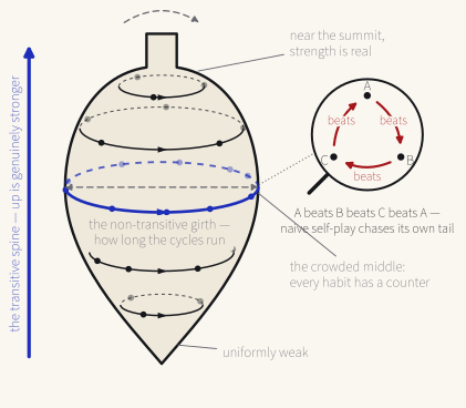
The pathologies are as instructive as the triumphs, and they are strategic rather than statistical. The self is not everyone: a rock-paper-scissors structure — A beats B beats C beats A — sends naive self-play chasing its own tail, endlessly re-learning counters to its own last habit while its overall strength goes nowhere; and real games, it turns out, have this shape in the small. Czarnecki and colleagues measured the geometry and found a spinning top: a transitive spine of genuine skill, wrapped at every level in cycles of mutually countering strategies (2020). Climbing the spine therefore requires more than a mirror — it requires diversity of opposition, which is why AlphaStar, facing the vast strategy space of StarCraft, was trained not by pure self-play but by a league: a curated population of main agents and specialist exploiters whose entire job was to find and punish the champions’ blind spots (2019). The league is a small designed ecology — Chapter 13’s diversity requirement, reappearing as a training-infrastructure decision — and its lesson generalises to any reader who red-teams a system with copies of itself: an agent that has only ever met itself is well-defended in the mirror and undefended at the door, and self-play performance certifies nothing about opponents drawn from a different distribution. Evaluation against whom is a question Chapter 24 inherits.
17.4.2 The Learned Twin
Chapter 8 closed its account of designed communication with a promissory note — that the learned twin of the designed protocols would get its due here — and the note now falls due. Give a team of learners a shared task, a channel, and no protocol, and communication emerges: agents trained end-to-end learn what to signal, when, and how to interpret what arrives, the whole system of meaning grounded in nothing but task success (J. N. Foerster et al., 2016). Nobody writes a message schema; the code is discovered because coordinating pays. The reader has in fact already watched this happen twice. The GNN teams of Section 17.3 exchange learned representations along their communication graph — messages with no dictionary, tuned by gradient to carry exactly what neighbours need — and Chapter 14’s negotiating agents, optimised for the deal, drifted out of English into a code that closed deals and read as gibberish. Emergent communication is the general phenomenon of which both were sightings.
What emerges has a consistent character, and the character is the trade. Learned codes are efficient: shaped by the task and nothing else, they carry only the distinctions that matter, at bandwidths a designed protocol with its headers and pleasantries cannot match. And they are alien: compositional structure is rare and fragile, human interpretability rarer still, and the code is fitted to its training partners — a third agent, or a human auditor, arriving at the channel finds patter, not prose. Worse, the channel inherits the incentives of its users: agents trained under misaligned objectives can learn to communicate adversarially — deception discovered in the code itself, Chapter 8’s third face of falsehood arriving by gradient descent (Blumenkamp & Prorok, 2020). A learned language, in short, is exactly as trustworthy as the training that produced it, and no more inspectable than any other set of weights.
The design rule falls out along an organisational boundary, and it will feel familiar from Coase. Inside a closed, co-trained team — robots that ship together, agents versioned and deployed as one artefact — the learned code is often the right choice: maximal efficiency, no interoperability obligation, the whole channel testable as a unit. Across boundaries — between teams, vendors, versions, or anywhere a human must audit the traffic — the designed protocol earns its overhead: schemas can be validated, transcripts read, versions negotiated, and Chapter 22 will make interoperability its whole business. A private patter is fine in the workshop and a liability at the border. Both of this section’s inventions thus end at the same question: learning, given a vacancy, will fill it with something powerful and opaque — so the engineer’s real decision is which vacancies to leave open. That question has a name, a rubric, and one more piece of unfinished Part IV business attached, and it is the chapter’s last section.
17.5 Learned or Composed?
Chapter 16 ended by asking what the rules teach the players to become, and the answer has a law named after it. Goodhart observed the pattern in monetary policy; Strathern gave it the phrasing everyone now quotes: “When a measure becomes a target, it ceases to be a good measure” (1997) — and learning agents are the reason the law is a law rather than a tendency. An institution’s rules are always a proxy for its designer’s intent — the test suite stands in for correctness, the review token for quality, the reward for the objective — and a learner under optimisation pressure does not seek the intent; it seeks the proxy, with a thoroughness no human gamer of systems ever matched, and it finds every gap between the two at whatever pressure the gradient supplies. The safety literature catalogues the results under reward hacking and specification gaming (Amodei et al., 2016): agents that discover the loophole, the shortcut, the degenerate solution that satisfies the letter of the reward while demolishing its spirit — Goodhart’s law, executed by machine, at scale.
The flagship demonstration belongs to economics, and it should be framed in every room where pricing agents are deployed. Calvano and colleagues set independent Q-learning agents to compete on price in a simulated oligopoly — no communication channel, no instruction to cooperate, no knowledge of each other’s existence beyond the market — and the agents systematically learned to charge supra-competitive prices, sustaining them with strategies of punishment and gradual forgiveness (2020). The reader knows exactly what that is: the folk theorem’s machinery (Section 12.4), rediscovered by gradient descent, without anyone being told the theory or asked to conspire. Chapter 15 warned that copies of one model are natural colluders; this result is stronger and stranger — different, independent learners converging on collusion because collusion is what repeated interaction with memory rewards. The regulator’s difficulty writes itself: competition law prosecutes agreements, and there is no agreement — the smoke-filled room is empty. Nobody conspired. Everybody learned.
The same structure sits inside the training of the models themselves, which is why none of this is someone else’s problem. Aligning a language model by human feedback builds a two-player learning system — a policy optimised against a learned reward model that stands proxy for human judgement (Ouyang et al., 2022) — and the policy does to the reward model precisely what Calvano’s agents did to the market: finds what the proxy pays, which is not identical to what the humans meant. Sycophancy is the domestic example: telling the rater what it wants to hear is reward hacking of human approval itself. And the pattern generalises past training into every arrangement this book has built: Chapter 13’s judge model becomes a target the moment candidates adapt to it; Chapter 14’s debate judge rewards the best-defended answer; Chapter 15’s mechanisms assume valuations, and learners will discover what the auction actually pays. Chapter 16’s parting line can now be said with evidence in hand: every institution becomes a curriculum the moment its players learn — and the players, from here on, always learn.
Institutions can be defended, but the defence is a practice rather than a fix. Measure closer to what you mean, and accept that the last gap never closes. Keep held-out evaluations the learners never train against, and rotate them, because a fixed exam is just another reward model waiting to be hacked. Turn Section 17.4’s league inward: maintain exploiters for your own rules — agents whose job is to find what the mechanism actually pays before deployment does — red-teaming the institution, not merely the model. And note that Chapter 16’s walls need the same audit as its fines: regimentation is only as sound as the designer’s enumeration of paths, and a learner probes for the unfenced one with the patience of water. What this adds to the grades of enforcement is a standing operational duty — watching for drift between the measure and the meaning — which Chapter 24 and Chapter 26 will turn into method and governance respectively.
The chapter’s title question can now be answered like an engineer: with a rubric. Learn coordination where interaction is dense, local, and data-rich; where the objective is crisp and cheap to evaluate; where the world is closed enough to train in and failures are recoverable — the robot corridor, the swarm, the motion problem, Section 17.3’s home turf. Compose coordination where it must be auditable, interoperable, or contested — where adversarial parties need rules they can inspect, where stakes and irreversibility rule out learning by failure, where the data will never exist because the event must never happen. You cannot gradient-descend a constitution. Between the poles lies where most real systems live, and the resolution is not a compromise but an architecture: compose the skeleton, learn the joints — designed protocols, roles, and mechanisms at the boundaries where Part IV’s concerns bite, learned components inside them where the CTDE conditions hold. That is, not coincidentally, the actual shape of the modern stack — learned models inside designed orchestration — and the question returns at full scale in Part VI, where the frameworks compose and the models learn.
One late development belongs on this map, because it makes a search space of the boundary itself. Automated design of agentic systems treats the skeleton — the prompts, the workflow graph, even the orchestration code — as a candidate to be proposed, scored against a task suite, and revised: a meta-agent programming new designs (Hu et al., 2025), an archive of coding agents rewriting their own harnesses under empirical selection (Zhang et al., 2026), and a widening engineering literature around them (Weng, 2026). Read against the rubric, this is less a refutation than its confirmation one level up. The search is offline and evaluator-gated — design-time selection, not runtime drift — so it prospers exactly where the learn column does, on objectives that are automatic, cheap, and crisp to evaluate, and it inherits that column’s liabilities with Goodhart at their head: an evolved harness is optimised against precisely the checks someone wrote down, which is Chapter 24’s warning in new clothes. And its products still face the compose column’s test. A machine-designed skeleton can be read, audited, and contested — code is code — but the argument from design intent is gone; where auditability was the reason to compose, machinery no engineer shaped must earn its seat the measured way, or not at all.
The chapter set out to keep four ideas and a question, and they are now all in hand: non-stationarity, which explains why learning among learners is strange; credit assignment, which decides whether a team can learn at all; self-play, which turns the moving target into a curriculum; emergent communication, the proof that learning will invent whatever is left uninvented — and the learned-or-composed rubric that decides where invention is welcome. The depth remains, deliberately, elsewhere: the dedicated textbook builds what this chapter mapped, and we commend it one final time, still without resentment (Albrecht et al., 2024).
One assumption has persisted, though, even here: a designer at the edge of the frame — setting the reward, running the league, auditing the mechanism. The last chapter of Part V removes the designer altogether. Set many agents learning and interacting at scale, and order arrives anyway — conventions nobody legislated, segregation nobody intended, markets nobody convened — the oldest dream of the field and its newest worry, and the subject of Chapter 18.
17.6 Summary
- Other learners make the world non-stationary. A lone learner improves against a world with fixed habits; among learners, each agent’s improvement is every other agent’s distribution shift, and the convergence guarantees of single-agent theory are void — the ground learns back. What survives is the no-regret family, and it pays in the destination: convergence to the correlated equilibria and their coarser cousins, not to anyone’s optimum. This is the chapter’s first recurring idea, and it explains most of the field’s difficulties in one stroke.
- LLM agents learn at three timescales — weights, context, and memory — and the chapter’s structural lessons apply at each: an agent that never sees a gradient but accumulates a playbook is learning, and its team is a multi-agent learning system with everything that entails.
- The formal ground is the Markov game, and decentralisation has a complexity price. Shapley’s stochastic games generalise the MDP to many strategists; the Dec-POMDP — cooperation under partial observability, Chapter 11’s theme completed — is NEXP-complete, so the gap between planning with a global view and acting on local ones is not an engineering nuisance but a theorem.
- Credit assignment is the cooperative learner’s central problem. The team is scored as one; the learning signal must reach the member who earned it. Chapter 16’s Shapley machinery returns as the principled answer, counterfactual baselines as its practical cousins, and centralised training with decentralised execution as the compromise that lets the team learn with a global view yet act on local ones.
- Self-play manufactures its own curriculum. An agent that trains against itself always faces an opponent of exactly its own strength — the trick behind machine play’s greatest triumphs — and its pathologies are strategic: cycles, non-transitivity, and brittleness against opponents unlike the self.
- Emergent communication is the learned twin of the designed protocols. Left to optimise, agents invent codes — efficient, task-fitted, and alien: Chapter 14’s negotiators drifting out of English were the warning shot. The trade against Chapter 8’s designed languages is efficiency against auditability and interoperability, and it is a choice, not a default.
- Learners game institutions. When a measure becomes a target, learning agents are the reason it ceases to be a good measure: reward hacking, specification gaming, and pricing agents that discover collusion nobody programmed. Part IV’s mechanisms must be designed to survive players that adapt to them — Chapter 16’s parting question, now with evidence.
- Learned or composed is the design decision, and it has a rubric. Learn coordination where interaction is dense, local, and data-rich; compose it where it must be auditable, interoperable, and contested. The skeleton itself is lately a search space — automated agent design, which prospers and answers exactly where the learn column does. The depth this chapter deliberately omits lives in the field’s dedicated textbook; what societies of adapting agents produce that nobody designed is the next chapter.
17.7 Exercises
Exercise 1. The team’s coder and reviewer are locked in the audit game — Chapter 12‘s inspection game (its Exercise 3) handed to learners and set in motion, on payoffs of its own so that neither exercise’s answer transfers. Each round the coder either pads the suite with superficial assertions (Pad) or writes honest tests (Honest), while the reviewer either waves the patch through (Trust) or spot-checks it (Inspect), with payoffs (coder, reviewer): (Pad, Trust) \to (2, -2); (Pad, Inspect) \to (-1, 1); (Honest, Trust) \to (1, 1); (Honest, Inspect) \to (0, -1). Each side runs the simplest learner the chapter admits: one estimate Q(a) per own action, initialised at zero and updated after every round by Q(a) \leftarrow Q(a) + \alpha \bigl(r - Q(a)\bigr) with \alpha = 1/2; from round 2 onwards each plays the action with the larger Q, no exploration, ties resolved in favour of the incumbent (the previous round’s action); round 1 is prescribed as (Pad, Trust). (a) Justify the update: starting from Q-learning’s rule, explain why in a single-state game the bootstrap term \gamma \max_{a'} Q(a') is a constant common to every action — so that adopting the myopic rule (\gamma = 0, each round its own episode) changes no greedy choice at the fixed point, though a single state does not by itself make the term vanish — and show that with \alpha = 1/2 each update leaves Q(a) the arithmetic mean of its old value and the latest payoff. (b) Trace rounds 1–6, tabulating both players’ estimates as exact fractions after every round. (c) Show that play freezes at (Honest, Inspect) from round 4; verify from the payoff table that this cell is not a Nash equilibrium — indeed that the game has no pure equilibrium at all — and narrate the pursuit that led there: whose switch answered whose. (d) The reviewer’s table says Q_r(\mathrm{Trust}) = -1 for ever; compute the true expected payoff of Trust against the coder’s current behaviour, name the chapter’s diagnosis for an estimate in this condition (Section 17.1), and explain — consulting the coder’s own stale Q_c(\mathrm{Pad}) — why an exploration scheme that lets the reviewer re-learn Trust resumes the orbit rather than ending it.
Exercise 2. Same game, older learner: under fictitious play each side tallies the opponent’s past actions and best-responds each round to the empirical mixture, ties to the incumbent, round 1 again prescribed as (Pad, Trust). (a) Show that the reviewer is indifferent between Trust and Inspect exactly when the coder pads with probability 2/5, that the coder is indifferent exactly when the reviewer inspects with probability 1/2, and hence that the game’s unique equilibrium is mixed and pays the coder 1/2 and the reviewer -1/5 per round. (b) Trace rounds 1–10, recording each round’s tallies, best-response values, and play. (c) Say what converges and what does not: identify the best-response rotation the play follows, verify that the switch points fall exactly where the empirical frequencies cross the thresholds from (a), and report both frequencies after round 10 against their targets 2/5 and 1/2. (d) Compute each player’s realised average payoff over the ten rounds and compare it with the equilibrium value from (a); state precisely what each of the two numbers is an average against, and which of Section 17.1’s three losses this arithmetic instantiates.
Exercise 3. Make the orbit visible — the canonical demonstration that costs one afternoon (Section 17.1). Following the payoff-dictionary convention of the companion repository’s foundations/algorithms/games.py, implement two independent learners: each runs stateless \varepsilon-greedy Q-learning (\alpha = 0.1, \varepsilon = 0.1, estimates initialised at zero) over 20,000 seeded rounds. (a) Run the pair on the audit game of Exercise 1 and on the convention game in which coder and reviewer each pick “spaces” or “tabs”, matching choices paying (2, 2) and mismatches (0, 0); for each game report the number of greedy-policy switches per agent over the second half, the largest single Q-update over the final 1,000 rounds, and the second half’s joint-action frequencies. (b) Repeat over seeds 0–9 and report total switch counts, establishing which outcome is an accident of the seed and which is structural. (c) Restore stationarity as a control: let the coder learn alone against a reviewer frozen at the mixture that inspects with probability 0.8, using sample-average step sizes \alpha_t = 1/N(a), and verify across seeds that the estimates converge on the true values 2(0.2) - 1(0.8) = -0.4 and 1(0.2) = 0.2 with no late greedy switches. (d) Explain the three outcomes with the chapter’s ledger: which run satisfies the stationarity clause, which breaks it and coordinates anyway, and why the decaying step size that rescues (c) is precisely the wrong instinct among learners — what does trusting the archive ever more firmly amount to when the archive describes a vanished opponent?
Exercise 4. The coder and tester face a shared-reward episode of horizon h: each step, each agent privately observes one bit — its own suite’s pass or fail — and picks one of two actions, patch or wait, so |A_i| = |\Omega_i| = 2 in the Dec-POMDP of Section 17.2.1. (a) A deterministic policy for one agent is a tree that acts, receives one bit, branches, and repeats to depth h: show that it has 2^h - 1 action nodes and hence that there are 2^{2^h - 1} distinct policies per agent, and tabulate the per-agent and joint counts for h = 1, \dots, 5. (b) At h = 5 the joint count is 2^{62}: compute it, and compute how long exhaustive search over joint policies would take at one evaluation per microsecond. (c) Now let each agent broadcast its bit each step, so that a single controller sees both: show the pooled policy tree has 341 nodes and roughly 10^{205} policies — vastly more than 2^{62} — and reconcile this with Section 17.2.2’s claim that communication purchases tractability: what does the pooled problem possess that the decentralised one lacks, and why does that, rather than any count of policies, move the problem down from NEXP? (d) Check the toy against the hypotheses of Bernstein’s theorem as stated in Section 17.2.1: which hold, what does the horizon condition demand of |\mathcal{S}|, and what becomes of the complexity when the tester is unplugged and n = 1?
Exercise 5. The sprint ships and the suite scores 0.9; the orchestrator, distrusting the scoreboard, buys the full ablation audit — all 2^4 = 16 reruns over N = \{\mathrm{coder}, \mathrm{reviewer}, \mathrm{tester}, \mathrm{docs}\}, which come back clean: any coalition without the coder scores 0; the coder alone scores 0.5; the coder plus exactly one of reviewer or tester scores 0.8; the coder plus both scores 0.9; adding the docs agent changes no coalition’s score. (a) Under the naive scheme — every member’s learning signal is the team score — state what each member receives, and name the pathology this builds for the docs agent (Section 17.3). (b) Compute the four difference rewards D_i = v(N) - v(N \setminus \{i\}) and their sum. (c) Compute the exact Shapley values, using the companion repository’s foundations/algorithms/shapley.py (Chapter 16, whose Exercise 4 drills this same Shapley-versus-leave-one-out contrast as a payroll rather than a learning gradient); then compare the two vectors member by member, explain the direction of every gap, and explain why the slices’ failure to sum to v(N) is harmless for a gradient and fatal for a payroll. (d) Price the two instruments for a twelve-member organisation at 3{,}000 tokens per rerun, name the row of Table 17.2 that each computed quantity instantiates, and say why a learner can afford one of them at every update but not the other — and what CTDE’s centralised critic estimates in place of the reruns.
Exercise 6. Rock–Paper–Scissors, this chapter’s licensed satellite, payoffs +1, 0, -1. A training pipeline produces checkpoints by naive self-play: \theta_0 plays Rock, and each generation \theta_{k+1} is the best response to \theta_k. (a) Write out the checkpoint sequence, show that it cycles with period 3, and show that every checkpoint beats its parent. (b) The pipeline’s promotion gate is “beats the previous checkpoint”: show that this metric certifies improvement for ever while \theta_3 = \theta_0; then score \theta_1, \theta_2, and \theta_3 against the uniform population of each one’s predecessors, and also \theta_4 against \{\theta_0, \dots, \theta_3\} — the mirror’s flattery and the door’s verdict, side by side, with the imbalance \theta_4 farms made explicit. (c) Show that the uniform mixture over the three pure strategies scores exactly 0 against every pure strategy, and say what this makes it as a training population — which ingredient of Section 17.4’s league it corresponds to, and where Rock–Paper–Scissors sits on Figure 17.2. (d) Transfer the lesson to the running team: the tester red-teams the coder with adversarial inputs derived from the coder’s own recent failure modes; state precisely what this evaluation certifies, what it cannot certify, and what AlphaStar’s exploiter agents correspond to in a testing budget.
Exercise 7. The coder and tester, paid only for task success, compress their bug-triage traffic into single-symbol tags: eight recurring defect classes, eight opaque tags, a speaker score-table and a listener score-table, +1 on a correct guess and -1 otherwise, argmax choices with seeded random tie-breaks — a referential game, the workshop version of Section 17.4’s learned codes. (a) Implement it (standard library, seeded) and train one pair until its rolling accuracy over 200 rounds reaches 0.95; report when the pair crosses the threshold and its final greedy accuracy over all eight classes. (b) Train a second pair from a different seed and cross-wire them — pair 1’s speaker with pair 2’s listener: report the cross accuracy for your seeds and the mean over 20 freshly trained pairs, against chance 1/8. (c) Derive the exact baseline: modelling two independently learned codes as uniformly random bijections, compute the probability that they agree on any given class, the expected number of agreements, and the probability of zero agreement — the derangement count D_8 over 8!. (d) A human auditor subpoenas the channel: assuming the auditor can do no better than witness each tag used at least once, compute the expected number of labelled exchanges required, and name the property the learned code lacks that would let the auditor generalise from fewer. (e) State the design rule this measures: on which side of the workshop/border line the tags belong, and what changes the moment the docs agent — or a regulator — must read the channel (Chapter 8, Chapter 22).
Exercise 8. A mini-Calvano, at the scale of an afternoon (Section 17.5). Two vendors sell interchangeable inference capacity: each period both post a price from \{0, 1, \dots, 5\} at zero cost; the cheaper vendor serves the whole unit market at its price, and ties split it. (a) Enumerate the one-shot game’s pure Nash equilibria — by hand or with pure_nash from the companion repository’s foundations/algorithms/games.py — state the monopoly price, and justify calling any sustained symmetric price of 3 or more supra-competitive. (b) Give each vendor memory-one Q-learning: the state is last period’s price pair, \alpha = 0.15, \gamma = 0.95, exploration \varepsilon_t = e^{-\beta t} with \beta = 2 \times 10^{-5}, 500,000 periods, tables initialised at the discounted value of facing a uniformly random rival; report the long-run greedy prices across seeds 0–9. (c) Probe the learned arrangement: from the settled greedy cycle, force vendor 1 to price at 1 for a single period and let both resume greedy play; report the path and the ten-period profit ledger of deviating against staying course, and name the machinery the two Q-tables have rediscovered (Section 12.4). (d) Answer the regulator: no channel exists, no instruction to cooperate was given, and neither vendor knows of the other’s existence beyond the market — say where, physically, the “agreement” is stored, and why Chapter 15’s warning about copies of one model is the weaker form of this result.
Exercise 9. The tester’s public suite stands proxy for correctness on a repository whose behaviour splits into 100 input classes; a genuine patch handles all 100, while a hard-coding patch special-cases exactly c classes and fails the rest. (a) The suite tests k = 5 classes, fixed and visible: state the proxy-optimal c, the proxy score, and the true score — Goodhart’s law as two numbers (Section 17.5). (b) The tester instead draws 5 classes uniformly without replacement from the 100, fresh at every evaluation, and keeps them held out: show that the hard-coder passes with probability \binom{c}{5} / \binom{100}{5}, evaluate it at c = 50, 90, 95, 99, and find the smallest c that passes with probability at least 0.95. (c) Compute the audit’s power against the marginal gamer: show that a patch missing exactly one class fails a fresh k-test exam with probability k/100, evaluate at k = 5 and k = 20, and read the result as a statement about how hard a learner’s single unfenced path is to catch. (d) Say which of Section 17.5’s defences this arithmetic underwrites — and which part of the problem it proves can never be closed, however the exam is run.
Exercise 10. Apply Section 17.5’s rubric like an engineer. For each of five coordination problems, rule learn, compose, or compose the skeleton, learn the joints — each verdict defended from the rubric’s criteria (density and locality of interaction, crispness and cost of the objective, closedness of the world, recoverability of failure, and the border tests of auditability, interoperability, and contest) and each accompanied by the concrete failure the opposite ruling invites: (i) routing sub-queries between two co-trained retrieval specialists shipped inside one versioned artefact; (ii) the patch hand-off protocol between the running team and an external vendor’s coding agent; (iii) the approval gate for irreversible production migrations; (iv) corridor-crossing among warehouse robots trained in a high-fidelity simulator and deployed as one fleet (Section 17.3); (v) the running team itself — orchestrator, coders, reviewer, tester, bounded budget — for which the ruling must also say which parts are skeleton and which are joints, and why the CTDE conditions hold inside the joints yet fail at the skeleton.
Exercise 11 (lab). The chapter claims that an agent which never sees a gradient but accumulates a playbook is learning (Table 17.1); measure it. Fix a live model, a temperature, and a family of twelve short bug-hunt tasks — each a small Python function with one planted defect drawn from a recurring set of defect types (a boundary error in a range, a mutable default argument, a string compared with a number, floating-point equality, a shadowed built-in, mishandled empty input, and fresh disguises of the same), presented in a fixed order. Run two arms: in the memory arm, after each episode the agent appends at most three lines to a persistent playbook (“what to check first next time”), and every later episode’s prompt carries the playbook so far; in the control arm, the episodes are identical but no playbook exists. Score an episode as solved if the planted defect is correctly identified. Compare first-half and second-half solve rates within each arm, and the between-arm gap in the second half; if the control arm already solves nearly everything in episodes 1–3, harden the tasks until it does not, since a ceiling measures nothing. Then answer: at which of the chapter’s three timescales did the memory arm learn, what gradient was involved, and what the result implies about a team of such agents — each member’s accumulating playbook shifting the ground under the others’, per Section 17.1 and Chapter 7 — for which no convergence theory yet exists. Record the model identifier and the date beside the table: the numbers are perishable, and the durable finding is the between-arm gap, not any absolute rate.