%%{init: {"theme": "base", "themeVariables": {"primaryColor": "#E8ECFF", "primaryBorderColor": "#4054B2", "primaryTextColor": "#16171B", "lineColor": "#3B4351", "edgeLabelBackground": "#FAF7F0", "clusterBkg": "#EFE9DC", "clusterBorder": "#766F65"}, "flowchart": {"rankSpacing": 26, "nodeSpacing": 32}}}%%
flowchart TB
  subgraph TRAIN["Training --- centralised"]
    direction LR
    G["Global state +<br/>joint actions"] --> K["Central critic"]
    K -->|"credit signal"| P1["π₁"]
    K --> P2["π₂"]
    K --> P3["π₃"]
  end
  subgraph EXEC["Execution --- decentralised"]
    direction TB
    O1["local obs o₁"] --> Q1["π₁"] --> A1["action a₁"]
    O2["o₂"] --> Q2["π₂"] --> A2["a₂"]
    O3["o₃"] --> Q3["π₃"] --> A3["a₃"]
    KX["✗ critic absent<br/>at execution"]
  end
  TRAIN ==>|"only the policies ship"| EXEC
  classDef world fill:#EFE9DC,stroke:#766F65,color:#16171B
  class KX world
14 Learning in Multi-Agent Systems
Part IV closed with its own confession: every institution it built was designed for players who stay put. This chapter withdraws the assumption, and everything changes character. A single agent learning alone faces a stationary problem, and theory rewards its patience; add one more learner and the guarantee quietly dies. Each agent’s training signal is now generated partly by the other’s behaviour, so each agent’s improvement is the other’s distribution shift: the coder learns to write what the reviewer approves, the reviewer learns new grounds for disapproval, and both aim at targets that move because they are being aimed at. The ground learns back. Everything distinctive about multi-agent learning follows from that one sentence.
“Learning” here happens at three timescales at once — the weights, the context, and the memory between them — the ledger of Table 14.1, drawn up in Section 14.1. The results were mostly discovered in the gradient world, but the structure — moving targets, credit to assign, curricula that generate themselves, rules that get gamed — recurs at all three, which is why the chapter is here.
The present twist is that the largest single-agent models are themselves products of multi-agent training — a policy and a reward model locked in their instructive little dance, models grading models. Multi-agent learning is no longer a corner of the field; it is the water. One stipulation, from the preface: this is a conceptual chapter — the book that teaches the algorithms properly already exists, is excellent, and is free. What this one keeps is the map: non-stationarity, credit assignment, self-play, and emergent communication — the learned twin of Chapter 5’s designed protocols — and the question Part VI will inherit: whether coordination among capable agents should be learned or composed.
14.1 Moving Targets: Learning Among Learners
Everything that makes learning alone tractable can be put in one sentence: the world does not care that you are learning. A lone agent improving by trial and error is running statistics on a process with fixed habits, and because the distributions hold still, improvement provably converges, under conditions the classical theory makes precise, on the best available. That theory — built on Bellman’s Markov Decision Process, met in Section 4.3 and deliberately not constructed here — rests every guarantee on one clause. The world may be stochastic, hostile, even unobservable; what it may not do is rearrange itself in response to being learned about.
That is exactly what another learner does. A second adapting agent is, from each agent’s chair, simply part of “the environment” — but an environment running the same manoeuvre in reverse: studying you, updating on you. The stationarity clause is broken by construction: in a system whose members adapt, everyone’s training data is generated by everyone else’s ongoing revision. This is non-stationarity: each agent is doing statistics on a data-generating process that its own statistics are changing. Whatever stability the system finds, it finds on its own.
The canonical demonstration costs one afternoon. Take a repeated two-player game, each player running standard single-agent learning and treating the other as scenery: what Tan called independent learners (1993). Sometimes this simply works — often enough to lull. And often it produces the signature pathology: pursuit. A adapts to B’s current habit; B revises; A’s estimates now describe an opponent that no longer exists, and the pair orbit the solution without settling, each perpetually well-adapted to the other’s recent past. The same disease afflicts learning from stored experience: a memory buffer of episodes against last week’s counterpart is archaeology — lovingly curated data about a vanished civilisation — and the more efficiently mined, the more precisely it fits what is gone. The chapter’s lab makes the orbit visible.
What breaks divides into three losses and one gain. The guarantees go first: convergence theorems condition on stationarity, so among learners they do not apply — not “apply more weakly”, do not apply. Evaluation goes next: “better” becomes opponent-indexed, so yesterday’s improvement can be today’s regression with nobody having blundered — a relativity Chapter 21 meets as a measurement problem and Section 14.4 as a strategic one. Third, legibility becomes a liability: an agent that adapts predictably can be farmed by a subtler learner — learning about learners is itself a game, Chapter 9’s business. The gain is the flip side: a target moving just ahead of the learner is a teacher, and arranging for it to move helpfully — curriculum by opponent — is the trick behind the field’s greatest successes (Section 14.4). The surveys organise around this ledger (Buşoniu et al., 2008); for the full taxonomy of remedies, go where the preface pointed — the field’s dedicated textbook (Albrecht et al., 2024), its Chapters 3 through 6 the natural companion syllabus — the first of several referrals, made without resentment.
One family of guarantees, essentially alone, survives the wreckage. An agent can bound its regret — the gap between what its choices earned and what the best fixed alternative would have earned in hindsight — against any opponent behaviour, because it never assumed a stationary world; and when every player learns under that discipline, the time-averaged joint play converges — not to Nash, but to the correlated equilibria or their coarser cousins, depending on the strength of regret driven down (Foster & Vohra, 1997; Hart & Mas-Colell, 2000). The pattern is this book’s thesis in miniature: what survives the passage from one agent to many is real, and always less than what was packed.
14.1.1 The Surviving Guarantee, Formally*
Fix a normal-form game \langle N, (A_i), (u_i) \rangle (Section A.4; A_i here are action sets), played repeatedly, and write a^{t} for the joint action at round t. Player i’s external regret after T rounds is
R_i^{T} \;=\; \max_{a \in A_i} \sum_{t=1}^{T} u_i\bigl(a, a^{t}_{-i}\bigr) \;-\; \sum_{t=1}^{T} u_i\bigl(a^{t}\bigr),
the gap between what its choices earned and what the best single action, held fixed for the whole history, would have earned against the same opponents; a learner is no-regret when R_i^{T}/T \to 0 whatever the opponents do. The collective destination is a property of the empirical distribution of play — the distribution \mu^{T} that weights each joint action by the fraction of the first T rounds spent there. Call a distribution \mu over joint actions a coarse correlated equilibrium when no player would rather commit to a fixed action than play along,
\mathbb{E}_{a \sim \mu}\bigl[u_i(a)\bigr] \;\ge\; \mathbb{E}_{a \sim \mu}\bigl[u_i(a', a_{-i})\bigr] \;\text{ for every } i \in N \text{ and } a' \in A_i,
and a correlated equilibrium — Aumann’s concept (1974) — when the inequality survives even deviations that see the draw: no relabelling f : A_i \to A_i achieves \mathbb{E}_{a \sim \mu}\bigl[u_i(f(a_i), a_{-i})\bigr] > \mathbb{E}_{a \sim \mu}\bigl[u_i(a)\bigr]. The everyday instance of the stronger concept is the traffic light: a public signal each driver conditions on, profitable to obey exactly because the others obey it. The concepts nest — a Nash equilibrium is a correlated equilibrium whose signal says nothing, the mixture being a product of independent randomisations — so Nash \subseteq correlated \subseteq coarse correlated, each inclusion generally strict.
The theorem the prose stated is now two lines long. If every player’s external regret grows sublinearly, any limit of the empirical distributions satisfies the displayed inequality — unfold the definitions and the average gain a fixed deviation a' would have collected is the per-round regret against a', so driving the one to zero extinguishes the other: play converges to the coarse correlated set, an observation as old as the no-regret analyses of the 1950s. Driving down the stronger swap regret — the same gap measured against every relabelling f — tightens the destination to the correlated equilibria (Foster & Vohra, 1997; Hart & Mas-Colell, 2000), and a general conversion turns any no-external-regret learner into a no-swap-regret one at modest cost (Blum & Mansour, 2007). The strength of regret buys the strength of the destination, which is the exact cash value of “or their coarser cousins” above.
None of this is quarantined in the gradient world — here the chapter earns its place. Our agents learn at three timescales (Table 14.1): the weights — training and fine-tuning, where the classical results live; the context — two agents in one conversation adapting to each other turn by turn, non-stationarity inside a single window; and between them the memory (Section 4.8) — a playbook accumulated and revised at deployment speed. A team of frozen-weight models with persistent memories is therefore a multi-agent learning system in every sense that matters — the coder’s accumulated style guide shifts what the reviewer sees, the reviewer’s remembered objections shift what the coder writes, the pair chasing each other’s revisions just as the Q-learners chase each other’s habits — and for memory-timescale learning there is, as yet, no convergence theory. The fastest timescale is a shade better served — in-context learning explained as implicit Bayesian inference or a step of gradient descent run in activations (Oswald et al., 2023; Xie et al., 2022), and first regret audits of LLM play (Park et al., 2025) — but all of it is single-agent so far. Engineers run these systems anyway; the gradient era’s structural lessons are the only map of this territory anyone has.
| Timescale | Cadence | Mechanism | Gradient? | Convergence theory |
|---|---|---|---|---|
| Weights | Slowest | Training and fine-tuning | Yes | Classical single-agent theory; among learners, only the no-regret family (Section 14.1) |
| Context | Fastest — turn by turn, within one window | Condition on the conversation so far (Chapter 2) | No | Nascent — single-agent accounts of in-context learning; first regret audits of LLM play |
| Memory | In between — one deployment at a time | Accumulate a playbook, retrieve precedents, revise one’s own notes (Section 4.8) | No | None, as yet |
14.2 The Formal Ground: Markov Games and the Dec-POMDP
The first remedy for a broken world model is a better one, in which other learners are not interference but inhabitants. A Markov game — Shapley called it a stochastic game, and defined it in 1953, the same remarkable year as his value (1953) — can be read in two directions: from Chapter 9 it is a matrix game given scenery — the joint action determines not only payoffs but the next state — and from the reinforcement-learning side it is an MDP given company, “the environment” containing other strategists by construction rather than by embarrassment. Shapley built the model to prove that zero-sum stochastic games have well-defined values, decades before anything resembling machine learning existed.
The frame’s first dividend is a taxonomy, for reward structure decides what “solving” means: fully cooperative games — every agent paid identically — pose a hard but well-posed team problem; two-player zero-sum games are Shapley’s clean original case, where the single-agent machinery generalises with dignity — Littman’s minimax-Q installed Markov games as the field’s standard frame by doing exactly that (1994); and general-sum games, almost everything real, import Chapter 9’s troubles wholesale — equilibria multiply, and “solving” quietly becomes “choosing which equilibrium to hope for”; what provably converges in a zero-sum game merely runs here.
The Markov game still assumes every player observes the whole board — and Chapter 8 spent its length on why teams do not. The model that takes both facts seriously — shared goal, joint dynamics, private views — is the Dec-POMDP: a decentralised, partially observable Markov decision process, in which a team earns a common reward while each member acts on nothing but its own history of private observations (Oliehoek & Amato, 2016). A policy here is not a plan over states — no agent has the state — but a mapping from private history to next action; communication, where it exists, is an action with a cost and a timing, not a free window onto teammates’ minds. This is the canonical mathematics of an orchestrated team.
Then the theorem that calibrates the enterprise. Bernstein and colleagues proved that solving a finite-horizon Dec-POMDP optimally is NEXP-complete (2002), and the scale deserves plain words (Section A.6 restocks the mantelpiece). NP-hard problems can at least have candidate solutions checked cheaply; single-agent partial observability is harder still — PSPACE-complete; NEXP sits above both, its brute-force cost doubly exponential — and the result holds for two agents, tiny horizons, everything finite and known. The jump from one decision-maker to two, under partial observability, is a change of complexity class — the price of decentralisation written as a theorem.
Why is two so much worse? The agents have lost the one thing that makes partial observability tractable alone: a shared summary of what is known. A single POMDP agent can maintain a belief state and act on it; a Dec-POMDP team has no common belief, so acting well requires reasoning about what teammates have seen, believe, and believe you have seen — Chapter 6’s nested beliefs, now the skeleton of the planning problem and the source of the second exponential. The Russian dolls, it turns out, were the complexity class.
14.2.1 The Markov Game and the Dec-POMDP, Formally*
The two frames deserve their tuples. A Markov game among n agents N = \{1, \dots, n\} is
\langle N, \mathcal{S}, \{A_i\}_{i \in N}, T, \{r_i\}_{i \in N}, \gamma \rangle,
where \mathcal{S} is the set of states; A_i is agent i’s action set, with joint actions A = A_1 \times \cdots \times A_n; T : \mathcal{S} \times A \to \Delta(\mathcal{S}) gives a probability distribution over next states, \Delta(X) denoting the set of probability distributions over X; r_i : \mathcal{S} \times A \to \mathbb{R} is agent i’s reward; and \gamma \in [0, 1) is the discount (reinforcement learning’s \gamma is the economics chapters’ \delta — both conventions are standard). The joint action is where the strategy lives: transitions and rewards answer to what everyone did. Set n = 1 and the tuple is Bellman’s MDP; shrink \mathcal{S} to a single state and it is one of Chapter 9’s repeated games — the section’s two readings of the model, recovered as special cases.
The Dec-POMDP amends this in three places, one informational, one motivational, and one clerical: each agent acquires a private observation set \Omega_i, with an observation function O : \mathcal{S} \times A \to \Delta(\Omega_1 \times \cdots \times \Omega_n) dealing every member its own partial glimpse of each state; the several rewards r_i merge into one shared r : \mathcal{S} \times A \to \mathbb{R}; and the discount \gamma goes, because the model will be run to a finite horizon rather than for ever — so that the whole reads
\langle N, \mathcal{S}, \{A_i\}_{i \in N}, T, r, \{\Omega_i\}_{i \in N}, O \rangle,
a team with common pay and private eyes. Since no agent sees the state, no agent can hold a policy over states: agent i’s policy is a map \pi_i : \Omega_i^{*} \to A_i from its private observation history — the sequence of everything it has personally seen — to its next action, and a joint policy is one such map per member. Bernstein’s theorem, with its hypotheses in full: given a Dec-POMDP over finite sets, with n \ge 2 agents, a finite horizon shorter than the number of states, and a threshold K, deciding whether any joint policy achieves expected total reward at least K is NEXP-complete (2002). Every hypothesis earns its keep — at n = 1 the same decision problem is PSPACE-complete; drop the short-horizon assumption and only the hardness half of the result survives; and note that this is only the decision version: certifying that a good enough joint policy exists already costs the class, and finding one is no cheaper.
14.2.2 Escape Routes
Hardness results are signposts, not stop signs: exact decentralised optimality being unattainable, everything practical buys the problem down, and the currencies are the themes of this book. Communication is the first: let the agents talk freely and cheaply and the team collapses towards a single centralised problem — merely PSPACE-hard; every message purchases tractability, Chapter 5 and Chapter 8’s machinery the purchasing. Offline centralisation is the second: execution must be decentralised, but preparation need not be — the CTDE compromise the next section examines. Pre-computed coordination is the third: Chapter 8’s conventions and Chapter 13’s roles are amortised planning, decided once, offline, outside anyone’s exponential. The theorem also exonerates the orchestrator: one coordinating context window is a rational escape from a complexity class.
What neither frame supplies is a signal: a cooperative team is scored as a team, and gradient or no gradient, the lesson has to reach the member whose behaviour earned it. That is credit assignment, and Chapter 13 has already supplied the instrument.
14.3 Whose Doing Was It? Credit and the CTDE Compromise
A cooperative team has one scoreboard; that is the problem. The sprint ships, the suite scores 84%, the whole team is paid the same number — and inside it, the coder’s elegant refactor and the reviewer’s afternoon of rubber-stamping are indistinguishable. Hand every member the global reward as its signal and the idle agent is reinforced whenever its colleagues succeed — free-riding by gradient, no cynicism required — the excellent agent punished for blunders it never made; and as the team grows, the correlation between one member’s behaviour and the shared outcome shrinks, so learning slows. This is multi-agent credit assignment, and it is Chapter 13’s fair-division question with the sentiment stripped out: not who deserves the reward, but where the gradient should land.
The principled answer is the one the reader already owns: Chapter 13’s Shapley value — but the offline audit is an afternoon, and a learner needs the quantity, or a serviceable shadow, at every step. The field’s workhorses are exactly such shadows (Table 14.2). Difference rewards ask the one-agent counterfactual — what would the team have scored had this agent stayed home? — and pay each member the difference, so free-riding earns precisely nothing (Wolpert & Tumer, 2001). COMA’s counterfactual baseline does the same surgery on actions rather than membership: marginalise out one agent’s action, everyone else’s held fixed, and credit the agent with how much its actual choice beat its average one (J. Foerster et al., 2018). Each is a single slice of the Shapley computation, evaluated cheaply where the full average cannot be; the practical art of cooperative learning is largely the art of estimating Chapter 13’s quantity at training-loop prices.
| Method | The counterfactual it asks | Cost | Slice of the Shapley audit |
|---|---|---|---|
| Shapley value (Chapter 13) | Marginal contribution, averaged over arrival orders | Exact — 16 runs for four agents, an afternoon; unaffordable per update | The full average |
| Difference rewards | What the team would have scored had this agent stayed home, or done something default | Cheap — affordable at every update | One slice, by membership |
| Counterfactual baseline (COMA) (J. Foerster et al., 2018) | How much better this agent’s action was than its average, others held fixed | Cheap — affordable at every update | One slice, by action |
Computing such counterfactuals requires seeing the whole board, and thereby hangs the field’s standard architecture. Centralised training with decentralised execution (CTDE) splits the agent’s life into two regimes (Figure 14.1): during training, a centralised critic observes the global state and every agent’s action — what makes counterfactual credit computable — while the policies being trained consume only their own local observations; at deployment the critic is dismantled like site scaffolding, and what ships is policies running on local views alone (J. Foerster et al., 2018; Lowe et al., 2017). This is Section 14.2’s cheque cashed — carefully, for it is smaller than it looks: centralising the training does not repeal NEXP-hardness; the global view buys the estimation, and a steadier target for the valuer — not the learners, who still train against teammates in motion. A related family factorises the team’s value into per-agent pieces so each member can act greedily on its own share (Rashid et al., 2018; Sunehag et al., 2018); at population scale — more pairwise relations than any critic can model — the joint value is rebuilt from pairwise interactions (Zhou et al., 2019) or every other learner summarised into a single mean neighbour (Yang et al., 2018), the crowd entering one agent’s problem as a field, not a roster — a way of seeing Chapter 15 will make general. CTDE is not a theorem but a compromise — the one on which most of modern cooperative multi-agent learning stands.
What the compromise can deliver, at its best, is coordination that was never written down anywhere. Prorok’s laboratory at Cambridge provides this book’s standing exhibit: teams of robots learn decentralised control policies structured as graph neural networks — each policy computes over its local neighbourhood, so the network architecture is the communication topology and the messages are the network’s own learned representations — trained centrally in simulation, executed on physical robots over ad-hoc radio (2022; 2020). The problems are Chapter 8’s own — the corridor, the crossing — but where Chapter 8 composed its solutions from locks, protocols, and conflict-based search, here the coordination is learned: nobody specified who yields, and the deference emerges in the weights — coordination with no protocol document, on hardware.
Heterogeneous teams — different sensors, bodies, jobs — sharpen the exhibit: one shared policy squanders the differences that make a team worth having, and training distinct policies that still coordinate is the harder problem the HetGPPO line addresses (Bettini et al., 2023) — a division of labour discovered by training, not assigned by charter. The ledger belongs beside the exhibit: learned coordination is data-hungry, simulation-bound until proven otherwise, and opaque in precisely the way composed coordination is not — no protocol document because no protocol, only weights. The ledger is the seed of Section 14.5’s rubric.
None of this is robotics parochialism: the credit problem does not care what the agents are made of. Fine-tune a multi-agent pipeline on team outcomes and the question is immediate: whose tokens get reinforced when the sprint ships? Reward every transcript equally and you have free-riding by gradient at the scale of a language model. At the memory timescale the same structure wears plain clothes: a team postmortem that praises or blames the right member — and updates the right playbook — is credit assignment in prose, with the offline ablation audit as its gold standard. The signal, then, can be fixed: counterfactual credit, centralised preparation, decentralised action. What remains unfixed is the moving target itself — and the field’s most productive discovery is that if the target is going to move anyway, you can choose what it is, and the best choice is frequently yourself.
14.4 What Learning Invents: Opponents and Languages
Leave a vacancy in a learning system’s world and, given enough gradient steps, the system will fill it. Supply no opponent, and learning builds one out of the only material to hand: itself. Supply no protocol, and a team that needs to talk invents a language nobody designed. These are the chapter’s third and fourth recurring ideas — self-play and emergent communication — the same phenomenon at different addresses: pressed, learning manufactures the missing parts of the game itself. Both produced some of the field’s most astonishing results, and both are the likeliest to hand an engineer something that works brilliantly and cannot be read.
14.4.1 Against Yourself
Self-play is the field’s most productive trick, its logic disarmingly simple: train an agent against copies of itself, and the moving target of Section 14.1 stops being a bug and becomes the syllabus. A fixed opponent teaches what it knows, then nothing; a random one teaches noise; an opponent always exactly your own strength — because it is you — delivers the perfect curriculum forever: never hopeless, never trivial, advancing at the learner’s pace. The origin story is Tesauro’s TD-Gammon, which taught itself backgammon to world-class strength and, along the way, revised human opening theory (1995).
The triumphs need no retelling, but their shape does. AlphaGo took human games as a foundation and self-play as the ascent (Silver et al., 2016); AlphaGo Zero removed the foundation, learning from nothing but the rules and its own play, and beat its predecessor soundly (2017) — an entire curriculum, from first flailing to superhuman strength, manufactured out of the rules plus a mirror. Self-play is non-stationarity harnessed. Nor is the manufactured opponent confined to games: the Generative Adversarial Network (GAN) builds one into the training objective — generator against discriminator, the forger improving because the detective does (Goodfellow et al., 2014) — and IRGAN carried the design to information retrieval, training a retrieval model against its generative adversary on exactly this pattern (Wang et al., 2017). The family’s notorious training instability travelled too — no accident: learners chasing each other are not obliged to settle.
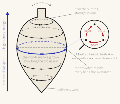
The pathologies are as instructive, and they are strategic rather than statistical. The self is not everyone: a rock-paper-scissors structure — A beats B beats C beats A — sends naive self-play chasing its own tail, and Czarnecki and colleagues found real games have this geometry: a spinning top, a transitive spine of genuine skill wrapped at every level in cycles of mutually countering strategies (2020) — Figure 14.2 draws it. Climbing the spine therefore requires diversity of opposition — hence AlphaStar’s league: a curated population of main agents and specialist exploiters whose job was to find and punish the champions’ blind spots (2019). The league is a designed ecology — Chapter 10’s diversity requirement as training infrastructure — and its lesson generalises to anyone who red-teams a system with copies of itself: an agent that has only ever met itself is well-defended in the mirror and undefended at the door.
14.4.2 The Learned Twin
Chapter 5 deferred the learned twin of communication to this chapter. Give a team of learners a shared task, a channel, and no protocol, and communication emerges: agents trained end-to-end learn what to signal, when, and how to interpret what arrives, meaning grounded in task success alone (J. N. Foerster et al., 2016) — no schema, the code discovered because coordinating pays. The reader has watched this twice already: Section 14.3’s GNN teams exchanging learned representations — messages with no dictionary — and Chapter 11’s negotiators drifting out of English into a code that closed deals and read as gibberish. Emergent communication is the general phenomenon; both were sightings.
What emerges has a consistent character, and it is the trade. Learned codes are efficient: shaped by the task and nothing else, they carry only the distinctions that matter. And they are alien: compositional structure rare, human interpretability rarer, the code fitted to its training partners — a third agent or human auditor arriving at the channel finds patter, not prose. Worse, the channel inherits its users’ incentives: agents trained under misaligned objectives can learn to communicate adversarially — deception discovered in the code itself, Chapter 5’s third face of falsehood arriving by gradient descent (Blumenkamp & Prorok, 2020). A learned language is exactly as trustworthy as the training that produced it, and no more inspectable than any other set of weights.
The design rule falls out along an organisational boundary, familiar from Coase. Inside a closed, co-trained team — robots that ship together, agents deployed as one artefact — the learned code is often right: maximal efficiency, no interoperability obligation, the channel testable as a unit. Across boundaries — between teams, vendors, versions, or wherever a human must audit the traffic — the designed protocol earns its overhead: schemas validated, transcripts read, versions negotiated, interoperability Chapter 19’s whole business. A private patter is fine in the workshop, a liability at the border. Both inventions end at the same question: learning, given a vacancy, will fill it with something powerful and opaque — so the engineer’s real decision is which vacancies to leave open. That is the chapter’s last section.
14.5 Learned or Composed?
Chapter 13 ended by asking what the rules teach the players to become, and the answer has a law named after it. Goodhart observed the pattern in monetary policy; Strathern gave it the quotable phrasing: “When a measure becomes a target, it ceases to be a good measure” (1997) — and learning agents are why it is a law rather than a tendency. An institution’s rules are always a proxy for its designer’s intent — the test suite stands in for correctness, the review token for quality, the reward for the objective — and a learner does not seek the intent; it seeks the proxy, and finds every gap. The safety literature files the results under reward hacking and specification gaming (Amodei et al., 2016): the loophole, the shortcut, the degenerate solution satisfying the letter of the reward while demolishing its spirit — Goodhart’s law, executed by machine, at scale.
The flagship demonstration belongs framed in every room where pricing agents are deployed. Calvano and colleagues set independent Q-learning agents — each keeping a table Q(s, a) of estimated long-run value and, after every step, nudging the entry it used a fraction \alpha of the way towards the reward plus \gamma times the best entry of the state it reached, Q(s,a) \leftarrow Q(s,a) + \alpha\bigl(r + \gamma \max_{a'} Q(s',a') - Q(s,a)\bigr) — competing on price in a simulated oligopoly — no channel, no instruction to cooperate, no knowledge of each other beyond the market — and the agents systematically learned supra-competitive prices, sustained by punishment and gradual forgiveness (2020). That is the folk theorem’s machinery (Section 9.4), rediscovered by gradient descent, nobody having been told the theory or asked to conspire. Chapter 12 warned that copies of one model are natural colluders; this is stronger and stranger — different, independent learners converging on collusion, because collusion is what repeated interaction with memory rewards. The regulator’s difficulty writes itself: competition law prosecutes agreements, and there is none — the smoke-filled room is empty. Nobody conspired. Everybody learned.
The same structure sits inside the training of the models themselves. Aligning a language model by human feedback builds a two-player learning system — a policy optimised against a learned reward model standing proxy for human judgement (Ouyang et al., 2022) — and the policy does to the reward model what Calvano’s agents did to the market: it finds what the proxy pays, not what the humans meant. The pattern generalises into every arrangement this book has built: Chapter 10’s judge model becomes a target the moment candidates adapt to it; Chapter 11’s debate judge rewards the best-defended answer; Chapter 12’s mechanisms assume valuations learners will see straight through. Chapter 13’s parting line now has evidence: every institution becomes a curriculum the moment its players learn — and the players, from here on, always learn.
Institutions can be defended, but the defence is a practice, not a fix. Measure closer to what you mean, accepting that the last gap never closes. Keep held-out evaluations the learners never train against, and rotate them — a fixed exam is just another reward model waiting to be hacked. Turn Section 14.4’s league inward: keep exploiters for your own rules, agents whose job is to find what the mechanism actually pays before deployment does. And Chapter 13’s walls need the same audit as its fines: regimentation is only as sound as the designer’s enumeration of paths, and a learner probes for the unfenced one with the patience of water. What this adds is a standing duty — watching for drift between measure and meaning — which Chapter 21 and Chapter 22 turn into method and governance.
The title question can now be answered like an engineer: with a rubric. Learn coordination where interaction is dense, local, and data-rich; where the objective is crisp and cheap to evaluate; where the world is closed enough to train in and failures recoverable — Section 14.3’s home turf. Compose coordination where it must be auditable, interoperable, or contested — where adversarial parties need inspectable rules, where stakes and irreversibility rule out learning by failure, where the data will never exist because the event must never happen. You cannot gradient-descend a constitution. Between the poles live most real systems, and the resolution is an architecture: compose the skeleton, learn the joints — Part III and Part IV’s protocols, roles, and mechanisms at the boundaries where their concerns bite, learned components inside them where the CTDE conditions hold. That is the shape of the modern stack, and the question returns at full scale in Part VI, where the frameworks compose and the models learn.
One late development makes the boundary itself a search space. Automated design of agentic systems treats the skeleton — prompts, workflow graph, even orchestration code — as a candidate to be proposed, scored against a task suite, and revised: a meta-agent programming new designs (Hu et al., 2025), coding agents rewriting their own harnesses under empirical selection (J. Zhang et al., 2026), a widening literature around them (Weng, 2026). Read against the rubric, this is confirmation one level up. The search is offline and evaluator-gated — design-time selection, not runtime drift — so it prospers where the learn column does and inherits its liabilities, Goodhart at their head: an evolved harness is optimised against precisely the checks someone wrote down, Chapter 21’s warning in new clothes. And its products still face the compose column’s test: a machine-designed skeleton can be read — code is code — but the argument from design intent is gone: machinery no engineer shaped must earn its seat the measured way, or not at all.
The joints’ side of the border is moving too. The substrate’s vendors now train models by reinforcement learning on agentic tasks themselves: an early exemplar fine-tuned a model to browse, search, and cite against a reward model of human preferences (Nakano et al., 2021); the practice has industrialised into tool-use and computer-use policies optimised against verifiable outcomes (G. Zhang et al., 2025). What this annexes is the inside of each seat: the plan–act–check scaffolding that prompt engineering used to compose arrives, increasingly, as a trained policy. But the annexation has a supply chain: the tasks and trajectories these policies train on come largely from composed systems — yesterday’s skeletons, instrumented and logged — so each advance of the joints is prepared by the composition above it. The harness is where coordination is practised before it can be trained, and the recurring prediction that scaffolding will be trained away entirely mistakes a ratchet for a countdown: every round of internalisation is fed by the composed practice it retires, and composition, by then, has moved up a floor. The rubric is unmoved — seams between parties stay composed because some seams must answer to someone — yet the joint share grows with every model generation, and an engineer should expect to re-draw the border each time the substrate moves — Chapter 18’s half-life discipline meeting this question from the other side.
The four ideas and the question are in hand; the depth remains, deliberately, elsewhere — the dedicated textbook builds what this chapter mapped, commended one final time, still without resentment (Albrecht et al., 2024).
One assumption has persisted even here: a designer at the edge of the frame — setting the reward, running the league, auditing the mechanism. The last chapter of Part V removes the designer. Set many agents learning and interacting at scale, and order arrives anyway — conventions nobody legislated, segregation nobody intended, markets nobody convened — the oldest dream of the field and its newest worry, and the subject of Chapter 15.
14.6 Summary
- Other learners make the world non-stationary. Each agent’s improvement is every other’s distribution shift, and single-agent convergence guarantees are void — the ground learns back. What survives is the no-regret family, and it pays in the destination: correlated equilibria, not anyone’s optimum.
- LLM agents learn at three timescales — weights, context, and memory — and the structural lessons apply at each: an agent that never sees a gradient but accumulates a playbook is learning, with everything that entails.
- The formal ground is the Markov game, and decentralisation has a complexity price. The Dec-POMDP — cooperation under partial observability — is NEXP-complete: the gap between planning globally and acting locally is a theorem, not a nuisance.
- Credit assignment is the cooperative learner’s central problem. The team is scored as one; the signal must reach the member who earned it. Shapley machinery returns as the principled answer, and CTDE is the compromise that made cooperative learning practical.
- Left to itself, learning invents opponents and languages. Self-play manufactures opponents always exactly one’s own strength — with pathologies of cycles and brittleness — and optimising agents invent codes that are efficient, task-fitted, and alien: efficiency against auditability, a choice, not a default.
- Learners game institutions, so learned or composed is the standing design decision. When a measure becomes a target, adapting agents are why it stops being a good measure; learn coordination where interaction is dense and data-rich, compose it where it must be auditable and contested — and the border is moving from both sides. What societies of adapting agents produce that nobody designed is the next chapter.
14.7 Exercises
Exercise 1. The team’s coder and reviewer are locked in the audit game — Chapter 9‘s inspection game (its Exercise 3) handed to learners and set in motion, on payoffs of its own so that neither exercise’s answer transfers. Each round the coder either pads the suite with superficial assertions (Pad) or writes honest tests (Honest), while the reviewer either waves the patch through (Trust) or spot-checks it (Inspect), with payoffs (coder, reviewer): (Pad, Trust) \to (2, -2); (Pad, Inspect) \to (-1, 1); (Honest, Trust) \to (1, 1); (Honest, Inspect) \to (0, -1). Each side runs the simplest learner the chapter admits: one estimate Q(a) per own action, initialised at zero and updated after every round by Q(a) \leftarrow Q(a) + \alpha \bigl(r - Q(a)\bigr) with \alpha = 1/2; from round 2 onwards each plays the action with the larger Q, no exploration, ties resolved in favour of the incumbent (the previous round’s action); round 1 is prescribed as (Pad, Trust). (a) Justify the update: starting from Q-learning’s rule, explain why in a single-state game the bootstrap term \gamma \max_{a'} Q(a') is a constant common to every action — so that adopting the myopic rule (\gamma = 0, each round its own episode) changes no greedy choice at the fixed point, though a single state does not by itself make the term vanish — and show that with \alpha = 1/2 each update leaves Q(a) the arithmetic mean of its old value and the latest payoff. (b) Trace rounds 1–6, tabulating both players’ estimates as exact fractions after every round. (c) Show that play freezes at (Honest, Inspect) from round 4; verify from the payoff table that this cell is not a Nash equilibrium — indeed that the game has no pure equilibrium at all — and narrate the pursuit that led there: whose switch answered whose. (d) The reviewer’s table says Q_r(\mathrm{Trust}) = -1 for ever; compute the true expected payoff of Trust against the coder’s current behaviour, name the chapter’s diagnosis for an estimate in this condition (Section 14.1), and explain — consulting the coder’s own stale Q_c(\mathrm{Pad}) — why an exploration scheme that lets the reviewer re-learn Trust resumes the orbit rather than ending it.
Exercise 2. Same game, older learner: under fictitious play each side tallies the opponent’s past actions and best-responds each round to the empirical mixture, ties to the incumbent, round 1 again prescribed as (Pad, Trust). (a) Show that the reviewer is indifferent between Trust and Inspect exactly when the coder pads with probability 2/5, that the coder is indifferent exactly when the reviewer inspects with probability 1/2, and hence that the game’s unique equilibrium is mixed and pays the coder 1/2 and the reviewer -1/5 per round. (b) Trace rounds 1–10, recording each round’s tallies, best-response values, and play. (c) Say what converges and what does not: identify the best-response rotation the play follows, verify that the switch points fall exactly where the empirical frequencies cross the thresholds from (a), and report both frequencies after round 10 against their targets 2/5 and 1/2. (d) Compute each player’s realised average payoff over the ten rounds and compare it with the equilibrium value from (a); state precisely what each of the two numbers is an average against, and which of Section 14.1’s three losses this arithmetic instantiates.
Exercise 3. Make the orbit visible — the canonical demonstration that costs one afternoon (Section 14.1). Following the payoff-dictionary convention of the companion repository’s foundations/algorithms/games.py, implement two independent learners: each runs stateless \varepsilon-greedy Q-learning (\alpha = 0.1, \varepsilon = 0.1, estimates initialised at zero) over 20,000 seeded rounds. (a) Run the pair on the audit game of Exercise 1 and on the convention game in which coder and reviewer each pick “spaces” or “tabs”, matching choices paying (2, 2) and mismatches (0, 0); for each game report the number of greedy-policy switches per agent over the second half, the largest single Q-update over the final 1,000 rounds, and the second half’s joint-action frequencies. (b) Repeat over seeds 0–9 and report total switch counts, establishing which outcome is an accident of the seed and which is structural. (c) Restore stationarity as a control: let the coder learn alone against a reviewer frozen at the mixture that inspects with probability 0.8, using sample-average step sizes \alpha_t = 1/N(a), and verify across seeds that the estimates converge on the true values 2(0.2) - 1(0.8) = -0.4 and 1(0.2) = 0.2 with no late greedy switches. (d) Explain the three outcomes with the chapter’s ledger: which run satisfies the stationarity clause, which breaks it and coordinates anyway, and why the decaying step size that rescues (c) is precisely the wrong instinct among learners — what does trusting the archive ever more firmly amount to when the archive describes a vanished opponent?
Exercise 4. The coder and tester face a shared-reward episode of horizon h: each step, each agent privately observes one bit — its own suite’s pass or fail — and picks one of two actions, patch or wait, so |A_i| = |\Omega_i| = 2 in the Dec-POMDP of Section 14.2.1. (a) A deterministic policy for one agent is a tree that acts, receives one bit, branches, and repeats to depth h: show that it has 2^h - 1 action nodes and hence that there are 2^{2^h - 1} distinct policies per agent, and tabulate the per-agent and joint counts for h = 1, \dots, 5. (b) At h = 5 the joint count is 2^{62}: compute it, and compute how long exhaustive search over joint policies would take at one evaluation per microsecond. (c) Now let each agent broadcast its bit each step, so that a single controller sees both: show the pooled policy tree has 341 nodes and roughly 10^{205} policies — vastly more than 2^{62} — and reconcile this with Section 14.2.2’s claim that communication purchases tractability: what does the pooled problem possess that the decentralised one lacks, and why does that, rather than any count of policies, move the problem down from NEXP? (d) Check the toy against the hypotheses of Bernstein’s theorem as stated in Section 14.2.1: which hold, what does the horizon condition demand of |\mathcal{S}|, and what becomes of the complexity when the tester is unplugged and n = 1?
Exercise 5. The tester’s public suite stands proxy for correctness on a repository whose behaviour splits into 100 input classes; a genuine patch handles all 100, while a hard-coding patch special-cases exactly c classes and fails the rest. (a) The suite tests k = 5 classes, fixed and visible: state the proxy-optimal c, the proxy score, and the true score — Goodhart’s law as two numbers (Section 14.5). (b) The tester instead draws 5 classes uniformly without replacement from the 100, fresh at every evaluation, and keeps them held out: show that the hard-coder passes with probability \binom{c}{5} / \binom{100}{5}, evaluate it at c = 50, 90, 95, 99, and find the smallest c that passes with probability at least 0.95. (c) Compute the audit’s power against the marginal gamer: show that a patch missing exactly one class fails a fresh k-test exam with probability k/100, evaluate at k = 5 and k = 20, and read the result as a statement about how hard a learner’s single unfenced path is to catch. (d) Say which of Section 14.5’s defences this arithmetic underwrites — and which part of the problem it proves can never be closed, however the exam is run.
Further exercises for this chapter continue in the web edition’s exercise bank.