%%{init: {"theme": "base", "themeVariables": {"primaryColor": "#E8ECFF", "primaryBorderColor": "#4054B2", "primaryTextColor": "#16171B", "lineColor": "#3B4351", "edgeLabelBackground": "#FAF7F0", "clusterBkg": "#EFE9DC", "clusterBorder": "#766F65"}, "flowchart": {"rankSpacing": 28, "nodeSpacing": 42, "subGraphTitleMargin": {"top": 4, "bottom": 14}}}}%%
flowchart TB
  subgraph WA ["World A"]
    CA(["Commander (loyal)"])
    L1A(["Lieutenant 1 (loyal)"])
    L2A(["Lieutenant 2 (traitor)"])
    CA -->|"attack (direct)"| L1A
    CA -->|"attack"| L2A
    L2A -->|"retreat (relayed)"| L1A
  end
  subgraph WB ["World B"]
    CB(["Commander (traitor)"])
    L1B(["Lieutenant 1 (loyal)"])
    L2B(["Lieutenant 2 (loyal)"])
    CB -->|"attack (direct)"| L1B
    CB -->|"retreat"| L2B
    L2B -->|"retreat (relayed)"| L1B
  end
  EQ["≡ same local view<br/>for Lieutenant 1"]
  L1A ~~~ CB
  L1A -.- EQ
  EQ -.- L1B
  classDef risk fill:#F4D7D5,stroke:#A4161A,color:#16171B
  classDef world fill:#EFE9DC,stroke:#766F65,color:#16171B
  class L2A,CB risk
  class EQ world
Appendix A — Mathematical Background
This appendix collects, in one place and one notation, the mathematics the book leans on. It is a refresher for the rusty and a reference for everyone else — not a course, and not a prerequisite: no chapter’s argument depends on anything here, because the book’s formal material lives beside its subject, in the starred sections, and this appendix keeps only the ground those sections stand on. Each section says what the ideas are, states the few results the book actually uses, and points to where they earn their keep. One chapter has a standing account to settle: Chapter 9 presents strategic interaction in prose and defers its formal machinery here, and Section A.4 honours the deferral — a deferral of statement, not of argument: the chapter’s case stands in its prose.
The notation is the book’s own — the same objects wear the same symbols here as in the chapters. There are n agents in the set N = \{1, \dots, n\}, indexed by i and j; probability is \Pr(\cdot) and expectation \mathbb{E}; tuples sit in angle brackets; \Delta(X) is the set of probability distributions over a finite set X; and the discount factor is \delta in the economics chapters and \gamma in the learning chapters, both conventions standard in their fields and neither willing to yield.
A.1 Probability, and the Arithmetic of Crowds
Nearly everything the book needs from probability is discrete and mercifully finite. A random variable X takes each of its possible values x with probability \Pr(X = x), the probabilities summing to one; its expectation is the probability-weighted average
\mathbb{E}[X] \;=\; \sum_{x} x \, \Pr(X = x),
and its variance, \mathrm{Var}(X) = \mathbb{E}\bigl[(X - \mathbb{E}[X])^{2}\bigr], measures the spread around it. Expectation is linear — the expectation of a sum is the sum of the expectations, with no conditions attached — which is why so many arguments in the book get away with adding averages.
Two events are independent when \Pr(A \text{ and } B) = \Pr(A)\Pr(B): learning that one occurred tells you nothing about the other. When it does tell you something, the conditional probability \Pr(A \mid B) = \Pr(A \text{ and } B) / \Pr(B) says how much, and Bayes’ rule turns the conditioning around,
\Pr(H \mid E) \;=\; \frac{\Pr(E \mid H) \, \Pr(H)}{\Pr(E)},
the arithmetic of updating a belief H on evidence E — the operation the Bayesian games of Section A.4 perform on opponents’ types, and the one calibration (Chapter 22) asks an agent’s confidence to have survived.
Run n independent trials, each succeeding with probability p, and the number of successes follows the binomial distribution: the probability of exactly k successes is
\binom{n}{k} \, p^{k} (1 - p)^{n - k},
which is the entire engine room of Section 10.4: the probability that a majority of n (odd) independent jurors is right is the upper tail of this distribution, the sum displayed there, and it is computed, not approximated. When a rate is wanted rather than the exact sum, one line of Hoeffding’s inequality prices the whole enterprise: for p > 1/2 the majority errs with probability at most e^{-2n(p - 1/2)^{2}} (Hoeffding, 1963) — error falling exponentially in the electorate, at a rate set by the square of the competence margin, so a jury built on half the margin must be four times the size for the same guarantee — and below one half the same exponent works for the prosecution, certainty of the wrong answer arriving at the same exponential speed. Behind it stands the law of large numbers — the mean \bar{x} of n independent observations of variance \sigma^{2} has variance \sigma^{2}/n, shrinking to nothing as the crowd grows — and behind the book’s endless fuss about diversity stands the same calculation with the independence removed. The calculation is short enough to carry in the pocket. The variance of a sum collects every pairwise interaction, a variance for each observation and a covariance for each ordered pair,
\mathrm{Var}(X_1 + \dots + X_n) \;=\; \sum_{i} \mathrm{Var}(X_i) \;+\; \sum_{i \ne j} \mathrm{Cov}(X_i, X_j),
so give the observations a common variance \sigma^{2} and a common nonnegative pairwise correlation \rho, making every covariance \rho\sigma^{2}: the right-hand side is n variance terms plus n(n-1) covariance terms, and dividing by n^{2} turns the sum into the mean,
\mathrm{Var}(\bar{x}) \;=\; \frac{n\sigma^{2} + n(n-1)\rho\sigma^{2}}{n^{2}} \;=\; \sigma^{2} \left[ \frac{1 - \rho}{n} + \rho \right],
whose first term the crowd washes out and whose second it cannot touch: averaging annihilates independent error completely and correlated error not at all, and no enlargement of the crowd changes the floor. The two ends of the dial say it plainest. At \rho = 0 the floor vanishes and the law of large numbers returns in full: \mathrm{Var}(\bar{x}) = \sigma^{2}/n, so a crowd of genuinely independent errors can be averaged down to any accuracy the budget will bear. At \rho = 1 it is the n that vanishes: \mathrm{Var}(\bar{x}) = \sigma^{2} however large the crowd, because observations that move as one are one observation, counted n times. And the count of terms explains why the middle of the dial matters so much more than the ends suggest: variances number n but covariances n(n-1), so as the crowd grows the correlation term does not merely persist, it takes over. That one formula is the mathematical content of the photocopied juror (Section 10.5), the correlated fleet (Section 15.5), and the caveat attached to the Byzantine bound below.
A.2 Statistics for Experimenters
Chapter 21’s discipline in one line is multiple runs or it did not happen; this section is the machinery that turns runs into conclusions. The sample mean \bar{x} of K independent measurements estimates the true mean; its own spread — the standard error — is s / \sqrt{K}, with s the sample standard deviation, and the working confidence interval is \bar{x} \pm 2s/\sqrt{K}: roughly 95% coverage, by the normal approximation that the averaging itself justifies for moderate K; for small K the multiplier comes from Student’s t instead — 2.57 at K = 6, 2.26 at K = 10, settling towards 1.96 — the correction Section 21.5’s six-task display pays. An effect is statistically distinguishable from chance when zero lies outside such an interval — equivalently, for the paired design of Section 21.5, when
t \;=\; \frac{\bar{d}}{s_d / \sqrt{K}}
is larger in magnitude than about two, \bar{d} and s_d being the mean and standard deviation of the per-task differences d_k defined there. The pairing matters more than the test: differencing on the same task cancels task difficulty before it can drown the signal. When the score is binary — pass or fail, the commonest agent metric — the paired instrument is McNemar’s test (McNemar, 1947): only the discordant tasks, those where the two systems disagree, carry any information, and the question reduces to whether A’s wins among them beat a fair coin. And a lone pass rate near either end of the scale outruns the two-standard-error approximation — at 18 passes in 20 the symmetric interval pokes above one — for which the Wilson interval is the standard repair (Wilson, 1927).
Two of Chapter 21’s cautions get their arithmetic here. Power: an interval built from too few tasks is simply wide, and a wide interval containing zero means we could not afford to know, not they are equal — absence of significance is not evidence of equality. Selection: pick the best of J configurations by noisy score and the winner’s measured advantage is inflated by construction; for roughly normal noise of size \sigma, the expected excess of the maximum of J pure-noise scores grows like
\sigma \sqrt{2 \ln J},
slowly but relentlessly — an asymptotic rate that flatters small fields: the exact figure at J = 8 is about 1.4\sigma, not the 2\sigma the formula suggests — which is why the winning configuration must be re-run on fresh tasks before its number is believed. Multiple testing is the same caution from the other side: run twenty tests at the 5% level and expect one false alarm even with nothing to find, and the blunt correction is to divide the significance level by the number of tests.
A.3 Utility, and What a Payoff Is
A utility function u represents an agent’s preferences when u(a) \ge u(b) exactly where the agent prefers a to b (or is indifferent). So understood, utility is bookkeeping, not a substance: any order-preserving relabelling of the numbers represents the same preferences, and nothing about a single agent’s utility scale supports comparison with anyone else’s.
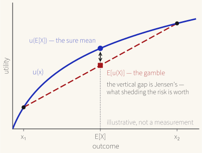
Risk changes that latitude. To choose among lotteries — outcomes delivered with probabilities — the standard is expected utility, \mathbb{E}[u(X)], and von Neumann and Morgenstern showed that an agent whose preferences over lotteries are consistent, in a precise and mild sense, behaves exactly as if maximising the expectation of some utility function (1944) — the result the whole payoff vocabulary of game theory rests on. The shape of u now carries meaning. A linear u values every gamble at its expectation and is called risk-neutral, the assumption under which Section 12.2’s revenue equivalence holds. A concave u rises ever more reluctantly, so that every chord sags below the curve, and the chord is the whole argument (Figure A.1): a fair coin-flip between a poor outcome x_1 and a good one x_2 is worth the average of the two utilities, the midpoint of the chord, while the sure average of the outcomes is worth the point on the curve directly above it. Jensen’s inequality says this once and in general: for concave u,
u\bigl(\mathbb{E}[X]\bigr) \;\ge\; \mathbb{E}\bigl[u(X)\bigr],
the sure mean worth at least the gamble, and the gap between the two sides is what shedding the risk is worth. An agent with such a u is risk-averse — the trait that breaks the equivalence, risk-averse bidders shading less under first-price rules, so that those formats then raise more (Section 12.2).
Mechanism design and coalitional theory add one further convenience: quasi-linear utility, u_i = v_i(x) - p_i — the value of the outcome minus the money paid — which makes money a common currency across agents. This is the “transferable value” the book flags in Chapter 12 and Chapter 13: it is what lets a mechanism price misrepresentation instead of forbidding it, and a coalition divide its spoils in any proportion. Where value cannot decently be made transferable, the impossibility results of Section 10.3 return in force. Time, finally, enters through discounting: a stream of payoffs u_0, u_1, u_2, \dots is valued at \sum_{t} \delta^{t} u_t for a discount factor \delta \in (0, 1), so that patience is a number — \delta near one — and the bargaining and repeated-game results of Section 11.2.1 and Section A.4 turn on how near one those numbers lie — and, in bargaining, on whose is nearer. One caution the book issues early and this appendix repeats: for artificial agents, utilities are not discovered but assigned — written by a designer, induced by a prompt, implied by an evaluation metric — and every theorem below computes faithfully from whatever was assigned (Section 12.1).
A.4 The Game-Theory Spine
What follows is the formal skeleton of Chapter 9, in the order that chapter tells the story; the standard full course is Osborne and Rubinstein (1994). It is the non-cooperative branch throughout — the coalitional theory that Chapter 13 develops is set aside here, and has a standard course of its own in Chakravarty, Mitra, and Sarkar (2015).
A.4.1 The Normal Form
A normal-form game is a tuple \langle N, (S_i)_{i \in N}, (u_i)_{i \in N} \rangle: the players N, a finite strategy set S_i for each, and payoff functions u_i assigning each profile s = (s_1, \dots, s_n) — one strategy per player, chosen simultaneously — a number for each player. The standing shorthand s_{-i} names everyone’s strategy but i’s, so a profile splits as (s_i, s_{-i}). A strategy s_i strictly dominates s_i' when u_i(s_i, s_{-i}) > u_i(s_i', s_{-i}) against every s_{-i}; weaken the inequality to \ge, holding strictly somewhere, and the dominance is weak — the grade truthful bidding achieves in Section 12.2. The Prisoner’s Dilemma of Section 9.1, in one standard numbering:
| Row \ Column | Cooperate | Defect |
|---|---|---|
| Cooperate | 3,\ 3 | 0,\ 5 |
| Defect | 5,\ 0 | 1,\ 1 |
A.4.2 Best Response and Equilibrium
Player i’s best response to s_{-i} is whatever serves it best given the others’ play, \mathrm{BR}_i(s_{-i}) = \operatorname*{arg\,max}_{s_i \in S_i} u_i(s_i, s_{-i}), and a Nash equilibrium is a profile in which the circle of anticipation closes — every player already best-responding to everyone else,
s^{*}_i \in \mathrm{BR}_i(s^{*}_{-i}) \;\text{ for every } i \in N,
so that no player gains by deviating alone. Set beside it the welfare standard: an outcome is Pareto-efficient if no alternative leaves some player better off and none worse. The two properties are independent — Section 9.2’s central warning — and the grid of Table A.1 is the proof by example: its only equilibrium is its only Pareto-dominated cell.
A.4.3 Mixed Strategies and Existence
Some games have no such resting point in definite choices — matching pennies punishes any predictable play — and the repair is randomisation: a mixed strategy is a distribution \sigma_i \in \Delta(S_i), payoffs extend by expectation, and best response and equilibrium read as before. Nash’s theorem is that every game with finitely many players and strategies has at least one equilibrium once mixtures are allowed (1950). Existence, however, is not reachability: computing a Nash equilibrium is PPAD-complete (Daskalakis et al., 2009), a class explained in Section A.6, and the gap between the two is a running theme of Chapter 9.
In the 2 \times 2 case, though, finding every equilibrium is a hand computation, and worth performing once in full. Take the Battle of the Sexes from Section 9.1’s field guide — two agents must adopt a single message schema, A is Row’s draft, B is Column’s, and any match beats none — in one standard numbering (Table A.2):
| Row \ Column | Schema A | Schema B |
|---|---|---|
| Schema A | 2,\ 1 | 0,\ 0 |
| Schema B | 0,\ 0 | 1,\ 2 |
The pure equilibria fall out of cell-by-cell inspection: at (A, A) either player’s unilateral switch drops its payoff to 0, so neither moves; (B, B) survives the same check; and at either mismatch each player gains by conforming, so both mismatches fail. That leaves the mixed equilibrium, and the workhorse that finds it: a player willingly randomises only between actions that pay it the same, so each player’s mixture is pinned by the other player’s indifference condition, not its own. Let Row play A with probability p. Column then expects p from playing A and 2(1-p) from playing B, and is indifferent exactly when p = 2(1-p): Row plays its own draft with probability p = 2/3. The matching condition on Column’s mixture q — Row expecting 2q from A and 1-q from B — gives q = 1/3, so each player favours its own schema two-thirds of the time. The price of the unbroken tie is then legible in the arithmetic: the players match with probability pq + (1-p)(1-q) = 4/9, and each expects 2/3 — less than the 1 that even the yielding player collects in either pure equilibrium, which is why Section 9.1 prescribes a convention with an accepted asymmetry rather than leaving both sides to their dice.
A.4.4 Sequence and Credibility
The extensive form replaces the grid with a tree: nodes where some player moves, branches for actions, payoffs at the leaves, and strategies promoted to complete contingent plans — an answer at every node of one’s own that could conceivably be reached. Solving the tree from its leaves upward is backward induction, and the refinement of Nash equilibrium it enforces is Selten’s subgame perfection: the strategies must form an equilibrium in every subgame, including the ones never reached on the equilibrium path (1965). That last clause is the formal content of Section 9.3’s campaign against empty threats — a threat is credible only if carrying it out would be rational at the node where it fires.
A.4.5 Repetition
Repeat a stage game indefinitely, discounting by \delta, and value a play by its discounted average payoff,
(1 - \delta) \sum_{t} \delta^{t} u_i(s^{t}),
the (1 - \delta) normalising the sum so that repeated-game payoffs live on the stage game’s own scale. The quantity that anchors what repetition can enforce is each player’s minmax value — the worst the others, randomising if they must, can hold player i to,
\underline{v}_i \;=\; \min_{\sigma_{-i}} \; \max_{s_i} \; u_i(s_i, \sigma_{-i}),
punishment, like unpredictability, sometimes needing the mixture — and since at any equilibrium player i is already best-responding to whatever the others play, no equilibrium can pay it less. The folk theorem is the converse at high patience: every feasible payoff profile — one achievable, on average, by some play, which is to say a point of the convex hull of the stage game’s payoff vectors — paying each player strictly more than its minmax can be sustained as a subgame-perfect equilibrium for \delta close enough to one, under a mild dimensionality condition on the feasible set (Fudenberg & Maskin, 1986). Note what it does and does not say — the sustainable set is enormous, containing the cooperative outcomes and any number of dreadful ones, which is exactly how Section 9.4 reads it: repetition enlarges the set of stable arrangements and declines to choose among them.
A.4.6 Incomplete Information
Harsanyi’s construction gives hidden motives a mathematics (1967). Endow each player with a type \theta_i \in \Theta_i bundling everything private — payoffs, abilities, information — let Nature draw the type profile from a common prior all players know, and let each observe only its own draw. A strategy becomes a plan per type, a map from \Theta_i to actions, and a Bayes–Nash equilibrium is a profile of such plans in which every type of every player best-responds in expectation, the expectation taken over the others’ types by Bayes’ rule (Section A.1) given the prior and their strategies. This is the formal home of Section 9.5 — and the working language of Chapter 12, whose auctions are Bayesian games somebody designed on purpose. Table A.3 gathers the spine’s solution concepts in one table.
| Concept | Game form | What it requires | Where the book uses it |
|---|---|---|---|
| Dominant strategy | Normal form | One strategy beats another against every opponent profile — strictly, or weakly if the edge holds strictly only somewhere | Prisoner’s Dilemma (Section 9.1); weak dominance grades truthful bidding (Section 12.2) |
| Nash equilibrium | Normal form | Every player best-responds to the others, so no one gains by deviating alone | Section 9.2 |
| Pareto efficiency (welfare standard) | Any outcome | No alternative leaves some player better off and none worse | Section 9.2 — set beside equilibrium, and deliberately independent of it |
| Mixed-strategy Nash equilibrium | Normal form with mixtures | Randomised best responses; guaranteed to exist by Nash’s theorem | Chapter 9 |
| Subgame-perfect equilibrium | Extensive form | A Nash equilibrium in every subgame, including those never reached on the equilibrium path | Section 9.3 |
| Folk-theorem equilibria | Repeated game | Any feasible payoff strictly above each player’s minmax, sustained for \delta close to one | Section 9.4 |
| Bayes–Nash equilibrium | Bayesian game (types, common prior) | Every type of every player best-responds in expectation over the others’ types | Section 9.5, Chapter 12 |
| Correlated equilibrium | Normal form with a shared signal | No player gains by deviating from its recommendation, even having seen it | Destination of swap-regret learners (Section 14.1.1) |
| Coarse correlated equilibrium | Normal form with a shared signal | No fixed deviation, chosen before the draw, profits against the distribution | Destination of no-regret learners (Section 14.1, Section 14.1.1) |
A.5 The Byzantine Bound
The result Section 20.13 states in prose is this. Suppose n parties must reach agreement while up to f of them are Byzantine: faulty in the worst way, free to lie, collude, and send different messages to different peers. Suppose too that messages are oral: delivered reliably and on schedule, so a silent sender is detectable, but carrying no proof of what anyone else said. Then, as Lamport, Shostak, and Pease proved (1982), agreement is achievable if and only if
n \;\ge\; 3f + 1,
strictly more than two-thirds of the council loyal. The impossibility half is a symmetry argument, visible already at n = 3, f = 1 (Figure A.2): a loyal lieutenant who hears “attack” from the commander and “he told me retreat” from the other lieutenant cannot tell a traitorous commander from a traitorous lieutenant — the two worlds present identically, so any rule it follows must obey the commander’s “attack” in both; the other loyal lieutenant, shown the mirror-image reports, is forced by the same rule to obey “retreat”; and in the world where the commander is the traitor, the two loyal lieutenants have thereby disagreed, which is the one thing agreement forbids. With n \ge 4 and one traitor, cross-checking majorities break the symmetry, and the general construction turns that into a protocol. Two caveats travel with the bound. Cryptographic signatures change the arithmetic — a signed message cannot be misquoted, and authenticated protocols tolerate more — and the bound is a count, not a probability: the traitors may collude as freely as they like, but there must be fewer than a third of them. As Section 20.9 insists, replicas that share one model do not fail one at a time; a single poisoned input can turn a thousand copies into a thousand traitors at once, so the premise that breaks is not independence, which the theorem never asked for, but the ceiling on f.
A.6 Complexity, Enough to Read the Signposts
The book quotes complexity classes the way sailors quote charts — not to prove anything, but to know where the water is deep — and reading the charts needs only a few conventions. The claims concern decision problems (yes/no questions), worst-case cost as the input grows, and reductions: a problem is hard for a class if every problem in the class translates into it cheaply, and complete if it is also a member — the class’s exact difficulty, in one specimen.
The ladder the book climbs: P, solvable in polynomial time; NP, checkable in polynomial time — a proposed solution can be verified cheaply, though finding one may not be — with NP-hardness the book’s workhorse warning, stamped on winner determination (Section 12.4), coalition structure generation (Section 13.1), optimal multi-agent path finding (Section 8.5), and even the manipulation of elections (Section 10.7, where it is conscripted as a shield (Bartholdi et al., 1989)); PSPACE, solvable in polynomial memory with unbounded time — the class of single-agent planning under partial observability (finite-horizon POMDPs are PSPACE-complete); and, one exponential up, EXP, solvable in exponential time, and NEXP, its checkable twin — certificates now exponentially long, brute force doubly exponential — so that the Dec-POMDP of Section 14.2.1 is its book-resident specimen. The containments run
\mathrm{P} \;\subseteq\; \mathrm{NP} \;\subseteq\; \mathrm{PSPACE} \;\subseteq\; \mathrm{EXP} \;\subseteq\; \mathrm{NEXP},
and the caveat is cheap: whether each adjacent inclusion is strict is open in every case, but the hierarchy theorems give \mathrm{P} \ne \mathrm{EXP} and \mathrm{NP} \ne \mathrm{NEXP}, so each long stretch of the chain genuinely climbs somewhere. That is enough to grade the jump Chapter 1 quotes for decentralising one decision-maker into two: a NEXP-complete problem provably lies beyond polynomial time, while a PSPACE-complete one, for all anyone has shown, need not — the move from one to the other crosses at least one boundary that is known to be real. One resident of the zoo is stranger and worth meeting: PPAD collects search problems whose solutions are guaranteed to exist by a fixed-point argument, so that the difficulty is purely one of finding; computing a Nash equilibrium is PPAD-complete (Daskalakis et al., 2009), which is how a resting point can be promised by Nash’s theorem and still lie beyond any efficient guarantee. Table A.4 sets the whole zoo out with each class’s book-resident specimen.
| Class | What it means | Where it bites in the book |
|---|---|---|
| P | Solvable in polynomial time | — |
| NP | Checkable in polynomial time — a proposed solution verifies cheaply, though finding one may not | Winner determination (Section 12.4), coalition structure generation (Section 13.1), optimal multi-agent path finding (Section 8.5), election manipulation as a shield (Section 10.7) |
| PSPACE | Solvable in polynomial memory with unbounded time | Single-agent planning under partial observability (finite-horizon POMDPs are PSPACE-complete) |
| EXP | Solvable in exponential time | — |
| NEXP | Checkable twin of EXP — certificates now exponentially long, brute force doubly exponential | The Dec-POMDP (Section 14.2.1) |
| PPAD | Search problems whose solution is guaranteed to exist by a fixed-point argument — only the finding is hard | Computing a Nash equilibrium (Section A.4) |
Read the signposts the way the book does. Hardness is a worst-case fact, not a forecast — real instances are often generous, which is how winner determination is solved to optimality in production (Section 12.4), and where generosity cannot be assumed, guarantees can still be bought, as when coalition search is bounded provably within a factor of optimal (Sandholm et al., 1999) — and a hardness result never says stop; it says stop looking for the free lunch. The moves it licenses are the ones the chapters actually make: centralise what would be intractable to decentralise (Section 14.2’s “rational escape from a complexity class”), approximate and pay the incentive bill knowingly (Section 12.3), or restructure the problem until the hard case no longer arises (Section 8.1’s designed-out dependency). That, in the end, is what this appendix is for: not to make the reader prove theorems, but to make the book’s signposts legible at driving speed.